ecterrab

14837 Reputation

24 Badges

21 years, 88 days

MaplePrimes Activity


These are Posts that have been published by ecterrab

The material below was presented in the "Semantic Representation of Mathematical Knowledge Workshop", February 3-5, 2016 at the Fields Institute, University of Toronto. It shows the approach I used for “digitizing mathematical knowledge" regarding Differential Equations, Special Functions and Solutions to Einstein's equations. While for these areas using databases of information helps (for example textbooks frequently contain these sort of databases), these are areas that, at the same time, are very suitable for using algorithmic mathematical approaches, that result in much richer mathematics than what can be hard-coded into a database. The material also focuses on an interesting cherry-picked collection of Maple functionality, that I think is beautiful, not well know, and seldom focused inter-related as here.


Digitizing of special functions,

differential equations,

and solutions to Einstein’s equations

within a computer algebra system


Edgardo S. Cheb-Terrab

Physics, Differential Equations and Mathematical Functions, Maplesoft

Editor, Computer Physics Communications


Digitizing (old paradigm)


• 

Big amounts of knowledge available to everybody in local machines or through the internet

• 

Take advantage of basic computer functionality, like searching and editing


Digitizing (new paradigm)

• 

By digitizing mathematical knowledge inside appropriate computational contexts that understand about the topics, one can use the digitized knowledge to automatically generate more and higher level knowledge


Challenges


1) how to identify, test and organize the key blocks of information,


2) how to access it: the interface,


3) how to mathematically process it to automatically obtain more information on demand


                                           Three examples


Mathematical Functions


"Mathematical functions, are defined by algebraic expressions. So consider algebraic expressions in general ..."

The FunctionAdvisor (basic)


"Supporting information on definitions, identities, possible simplifications, integral forms, different types of series expansions, and mathematical properties in general"

Examples


General description


References


Differential equation representation for generic nonlinear algebraic expressions - their use


"Compute differential polynomial forms for arbitrary systems of non-polynomial equations ..."

The Differential Equations representing arbitrary algebraic expresssions


Deriving knowledge: ODE solving methods


Extending the mathematical language to include the inverse functions


Solving non-polynomial algebraic equations by solving polynomial differential equations


References


Branch Cuts of algebraic expressions


"Algebraically compute, and visualize, the branch cuts of arbitrary mathematical expressions"

Examples


References


Algebraic expresssions in terms of specified functions


"A conversion network for arbitrary mathematical expressions, to rewrite them in terms of different functions in flexible ways"

Examples


General description


References


Symbolic differentiation of algebraic expressions


"Perform symbolic differentiation by combining different algebraic techniques, including functions of symbolic sequences and Faà di Bruno's formula"

Examples


References


Ordinary Differential Equations


"Beyond the concept of a database, classify an arbitrary ODE and suggest solution methods for it"

General description


Examples


References


Exact Solutions to Einstein's equations


Lambda*g[mu, nu]+G[mu, nu] = 8*Pi*T[mu, nu]


"The authors of "Exact solutions toEinstein's equations" reviewed more than 4,000 papers containing solutions to Einstein’s equations in the general relativity literature, organized the whole material into chapters according to the physical properties of these solutions. These solutions are key in the area of general relativity, are now all digitized and become alive in a worksheet"


The ability to search the database according to the physical properties of the solutions, their classification, or just by parts of keywords (old paradigm) changes the game.

More important, within a computer algebra system this knowledge becomes alive (new paradigm).

• 

The solutions are turned active by a simple call to one commend, called the g_  spacetime metric.

• 

Everything else gets automatically derived and set on the fly ( Christoffel symbols  , Ricci  and Riemann  tensors orthonormal and null tetrads , etc.)

• 

Almost all of the mathematical operations one can perform on these solutions are implemented as commands in the Physics  and DifferentialGeometry  packages.

• 

All the mathematics within the Maple library are instantly ready to work with these solutions and derived mathematical objects.


Finally, in the Maple PDEtools package , we have all the mathematical tools to tackle the equivalence problem around these solutions.

Examples


References


Download:  Digitizing_Mathematical_Information.mw,    Digitizing_Mathematical_Information.pdf

Edgardo S. Cheb-Terrab
Physics, Differential Equations and Mathematical Functions, Maplesoft

This presentation is on an undergrad intermediate Quantum Mechanics topic. Tackling the problem within a computer algebra worksheet in the way shown below is actually the novelty, using the Physics package to formulate the problem with quantum operators and related algebra rules in tensor notation.


Quantization of the Lorentz Force


Pascal Szriftgiser1 and Edgardo S. Cheb-Terrab2 

(1) Laboratoire PhLAM, UMR CNRS 8523, Université Lille 1, F-59655, France

(2) Maplesoft


We consider the case of a quantum, non-relativistic, particle with mass m and charge q evolving under the action of an arbitrary time-independent magnetic field "B=Curl(A(x,y,z)), "where `#mover(mi("A",mathcolor = "olive"),mo("→"))` is the vector potential. The Hamiltonian for this system is

H = (`#mover(mi("p",mathcolor = "olive"),mo("→"))`-q*`#mover(mi("A",mathcolor = "olive"),mo("→"))`(X))^2/(2*m)

where `#mover(mi("p",mathcolor = "olive"),mo("→"))` is the momentum of the particle, and the force acting in this particle, also called the Lorentz force, is given by


`#mover(mi("F",mathcolor = "olive"),mo("→"))` = m*(diff(v(t), t))


where `#mover(mi("v",mathcolor = "olive"),mo("→"))` is the quantized velocity of the particle, and all of  H, `#mover(mi("p",mathcolor = "olive"),mo("→"))`, `#mover(mi("v",mathcolor = "olive"),mo("→"))`, `#mover(mi("B",mathcolor = "olive"),mo("→"))`, `#mover(mi("A",mathcolor = "olive"),mo("→"))` and `#mover(mi("F",mathcolor = "olive"),mo("→"))` are Hermitian quantum operators representing observable quantities.


In the classic (non-quantum) case, `#mover(mi("F"),mo("→"))` for such a particle in the absence of electrical field is given by


`#mover(mi("F"),mo("→"))` = `&x`(q*`#mover(mi("v"),mo("→"))`, `#mover(mi("B"),mo("→"))`) ,


Problem: Departing from the Hamiltonian, show that in the quantum case the Lorentz force is given by [1]


`#mover(mi("F",mathcolor = "olive"),mo("→"))` = (1/2)*q*(`&x`(`#mover(mi("v",mathcolor = "olive"),mo("→"))`, `#mover(mi("B",mathcolor = "olive"),mo("→"))`)-`&x`(`#mover(mi("B",mathcolor = "olive"),mo("→"))`, `#mover(mi("v",mathcolor = "olive"),mo("→"))`))


[1] Photons et atomes, Introduction à l'électrodynamique quantique, p. 179, Claude Cohen-Tannoudji, Jacques Dupont-Roc et Gilbert Grynberg - EDP Sciences janvier 1987.


Solution


We choose to tackle the problem in Heisenberg's picture of quantum mechanices, where the state of a system is static and only the quantum operators evolve in time according to

``

diff(O(t), t) = I*Physics:-Commutator(H, O(t))/`ℏ`


Also, the algebraic manipulations are simpler using tensor abstract notation instead of the standard 3D vector notation. We then start setting the framework for the problem, a system of coordinates X, indicating the dimension of the tensor space to be 3 and the metric Euclidean, and that we will use lowercaselatin letters to represent tensor indices. In addition, not necessary but for convenience, we set the lowercase latin i to represent the imaginary unit and we request automaticsimplification so that the output of everything comes automatically simplified in size.


> 

restart; with(Physics); interface(imaginaryunit = i)

> 

Setup(mathematicalnotation = true, automaticsimplification = true, coordinates = X, dimension = 3, metric = Euclidean, spacetimeindices = lowercaselatin, quiet)

[automaticsimplification = true, coordinatesystems = {X}, dimension = 3, mathematicalnotation = true, metric = {(1, 1) = 1, (2, 2) = 1, (3, 3) = 1}, spacetimeindices = lowercaselatin]

(1)


Next we indicate the letters we will use to represent the quantum operators with which we will work, and also the standard commutation rules between position and momentum, always the starting point when dealing with quantum mechanics problems


> 

Setup(quantumoperators = {F}, hermitianoperators = {A, B, H, p, r, v, x}, realobjects = {`ℏ`, m, q}, algebrarules = {%Commutator(p[k], p[n]) = 0, %Commutator(x[k], p[l]) = I*`ℏ`*KroneckerDelta[k, l], %Commutator(x[k], x[l]) = 0})

[algebrarules = {%Commutator(p[k], p[n]) = 0, %Commutator(x[k], p[l]) = I*`ℏ`*Physics:-KroneckerDelta[k, l], %Commutator(x[k], x[l]) = 0}, hermitianoperators = {A, B, H, p, r, v, x}, quantumoperators = {A, B, F, H, p, r, v, x}, realobjects = {`ℏ`, m, q, x1, x2, x3, %dAlembertian, Physics:-dAlembertian}]

(2)


Note that we start not indicating F as Hermitian, in order to arrive at that result. The quantum operators A, B, and F are explicit functions of X, so to avoid redundant display of this functionality on the screen we use


> 

CompactDisplay((A, B, F)(X))

A(x1, x2, x3)*`will now be displayed as`*A


B(x1, x2, x3)*`will now be displayed as`*B


F(x1, x2, x3)*`will now be displayed as`*F

(3)

Define now as tensors the quantum operators that we will use with tensorial notation (recalling: for these, Einstein's sum rule for repeated indices will be automatically applied when simplifying)


> 

Define(x, p, v, A, B, F, quiet)

{A, B, F, p, v, x, Physics:-Dgamma[a], Physics:-Psigma[a], Physics:-d_[a], Physics:-g_[a, b], Physics:-KroneckerDelta[a, b], Physics:-LeviCivita[a, b, c], Physics:-SpaceTimeVector[a](X)}

(4)

The Hamiltonian,

H = (`#mover(mi("p",mathcolor = "olive"),mo("→"))`-q*`#mover(mi("A",mathcolor = "olive"),mo("→"))`(X))^2/(2*m)

in tensorial notation, is given by

> 

H = (p[n]-q*A[n](X))^2/(2*m)

H = (1/2)*Physics:-`^`(p[n]-q*A[n](X), 2)/m

(5)

Generally speaking to arrive at  ```#mover(mi("F",mathcolor = "olive"),mo("→"))` = (1/2)*q*(`&x`(`#mover(mi("v",mathcolor = "olive"),mo("→"))`, `#mover(mi("B",mathcolor = "olive"),mo("→"))`)-`&x`(`#mover(mi("B",mathcolor = "olive"),mo("→"))`, `#mover(mi("v",mathcolor = "olive"),mo("→"))`)) what we now need to do is

1) Express this Hamiltonian (5) in terms of the velocity


And, recalling that, in Heisenberg's picture, quantum operators evolve in time according to

diff(O(t), t) = I*Physics:-Commutator(H, O(t))/`ℏ`


2) Take the commutator of H with the velocity itself to obtain its time derivative and, from `#mover(mi("F",mathcolor = "olive"),mo("→"))` = m*(diff(v(t), t)) , that commutator is already the force up to some constant factors.


To get in contact with the basic commutation rules between position and momentum behind quantum phenomena, the quantized velocity itself can be computed as the time derivative of the position operator, i.e as the commutator of x[k] with H

> 

I*Commutator(H = (1/2)*Physics[`^`](p[n]-q*A[n](X), 2)/m, x[k])/`ℏ`

I*Physics:-Commutator(H, x[k])/`ℏ` = (1/2)*(I*q^2*Physics:-AntiCommutator(A[n](X), Physics:-Commutator(A[n](X), x[k]))-I*q*Physics:-AntiCommutator(p[n], Physics:-Commutator(A[n](X), x[k]))-2*(q*A[n](X)-p[n])*Physics:-KroneckerDelta[k, n]*`ℏ`)/(`ℏ`*m)

(6)

This expression for the velocity, that involves commutators between the potential A[n](X), the position x[k] and the momentum p[n], can be simplified taking into account the basic quantum algebra rules between position and momentum. We assume that A[n](X)(X) can be decomposed into a formal power series (possibly infinite) of the x[k], hence all the A[n](X) commute between themselves as well as with all the x[k]


> 

{%Commutator(A[k](X), x[l]) = 0, %Commutator(A[k](X), A[l](X)) = 0}

{%Commutator(A[k](X), x[l]) = 0, %Commutator(A[k](X), A[l](X)) = 0}

(7)

(Note: in some cases, this is not true, but those cases are beyond the scope of this worksheet.)


Add these rules to the algebra rules already set so that they are all taken into account when simplifying things


> 

Setup(algebrarules = {%Commutator(A[k](X), x[l]) = 0, %Commutator(A[k](X), A[l](X)) = 0})

[algebrarules = {%Commutator(p[k], p[n]) = 0, %Commutator(x[k], p[l]) = I*`ℏ`*Physics:-KroneckerDelta[k, l], %Commutator(x[k], x[l]) = 0, %Commutator(A[k](X), x[l]) = 0, %Commutator(A[k](X), A[l](X)) = 0}]

(8)
> 

Simplify(I*Physics[Commutator](H, x[k])/`ℏ` = (1/2)*(I*q^2*Physics[AntiCommutator](A[n](X), Physics[Commutator](A[n](X), x[k]))-I*q*Physics[AntiCommutator](p[n], Physics[Commutator](A[n](X), x[k]))-2*(q*A[n](X)-p[n])*Physics[KroneckerDelta][k, n]*`ℏ`)/(`ℏ`*m))

I*Physics:-Commutator(H, x[k])/`ℏ` = (-A[k](X)*q+p[k])/m

(9)

The right-hand side of (9) is then the kth component of the velocity tensor quantum operator, the relationship is the same as in the classical case

> 

v[k] = rhs(I*Physics[Commutator](H, x[k])/`ℏ` = (-A[k](X)*q+p[k])/m)

v[k] = (-A[k](X)*q+p[k])/m

(10)

and with this the Hamiltonian (5) can now be rewritten in term of the velocity completing step 1)

> 

simplify(H = (1/2)*Physics[`^`](p[n]-q*A[n](X), 2)/m, {SubstituteTensorIndices(k = n, (rhs = lhs)(v[k] = (-A[k](X)*q+p[k])/m))})

H = (1/2)*m*Physics:-`^`(v[n], 2)

(11)

For step 2), to compute

 `#mover(mi("F",mathcolor = "olive"),mo("→"))` = m*(diff(v(t), t)) and m*(diff(v(t), t)) = I*m*Physics:-Commutator(H, v(t)[k])/`ℏ` 


we need the commutator between the different components of the quantized velocity which, contrary to what happens in the classical case, do not commute. For this purpose, take the commutator between (10) with itself after replacing the free index

> 

Commutator(v[k] = (-A[k](X)*q+p[k])/m, SubstituteTensorIndices(k = n, v[k] = (-A[k](X)*q+p[k])/m))

Physics:-Commutator(v[k], v[n]) = -q*(Physics:-Commutator(A[k](X), p[n])+Physics:-Commutator(p[k], A[n](X)))/m^2

(12)

To simplify (12), we use the fact that if f  is a commutative mapping that can be decomposed into a formal power series in all the complex plan (which is assumed to be the case for all A[n](X)(X)), then

Physics:-Commutator(p[k], f(x, y, z)) = -I*`ℏ`*`∂`[k](f(x, y, z))

where p[k]"=-i `ℏ` `∂`[k] " is the momentum operator along the x[k] axis. This relation reads in tensor notation:

> 

Commutator(p[k], A[n](X)) = -I*`ℏ`*d_[k](A[n](X))

Physics:-Commutator(p[k], A[n](X)) = -I*`ℏ`*Physics:-d_[k](A[n](X), [X])

(13)

Add this rule to the rules previously set in order to automatically take it into account in (12)

> 

Setup(Physics[Commutator](p[k], A[n](X)) = -I*`ℏ`*Physics[d_][k](A[n](X), [X]))

[algebrarules = {%Commutator(p[k], p[n]) = 0, %Commutator(p[k], A[n](X)) = -I*`ℏ`*Physics:-d_[k](A[n](X), [X]), %Commutator(x[k], p[l]) = I*`ℏ`*Physics:-KroneckerDelta[k, l], %Commutator(x[k], x[l]) = 0, %Commutator(A[k](X), x[l]) = 0, %Commutator(A[k](X), A[l](X)) = 0}]

(14)
> 

Physics[Commutator](v[k], v[n]) = -q*(Physics[Commutator](A[k](X), p[n])+Physics[Commutator](p[k], A[n](X)))/m^2

Physics:-Commutator(v[k], v[n]) = -I*q*`ℏ`*(Physics:-d_[n](A[k](X), [X])-Physics:-d_[k](A[n](X), [X]))/m^2

(15)

Also add this other rule so that it is taken into account automatically

> 

Setup(Physics[Commutator](v[k], v[n]) = -I*q*`ℏ`*(Physics[d_][n](A[k](X), [X])-Physics[d_][k](A[n](X), [X]))/m^2)

[algebrarules = {%Commutator(p[k], p[n]) = 0, %Commutator(p[k], A[n](X)) = -I*`ℏ`*Physics:-d_[k](A[n](X), [X]), %Commutator(v[k], v[n]) = -I*q*`ℏ`*(Physics:-d_[n](A[k](X), [X])-Physics:-d_[k](A[n](X), [X]))/m^2, %Commutator(x[k], p[l]) = I*`ℏ`*Physics:-KroneckerDelta[k, l], %Commutator(x[k], x[l]) = 0, %Commutator(A[k](X), x[l]) = 0, %Commutator(A[k](X), A[l](X)) = 0}]

(16)

Recalling now the expression of the Hamiltonian (11) as a function of the velocity, one can compute the components of the force operator  "()Component(v*B,k)=m (v[k])=(i m [H,v[k]][-])/`ℏ`"

> 

F[k](X) = I*m*%Commutator(rhs(H = (1/2)*m*Physics[`^`](v[n], 2)), v[k])/`ℏ`

F[k](X) = I*m*%Commutator((1/2)*m*Physics:-`^`(v[n], 2), v[k])/`ℏ`

(17)

Simplify this expression for the quantized force taking the quantum algebra rules (16) into account

> 

Simplify(F[k](X) = I*m*%Commutator((1/2)*m*Physics[`^`](v[n], 2), v[k])/`ℏ`)

F[k](X) = (1/2)*q*(-Physics:-`*`(Physics:-d_[n](A[k](X), [X]), v[n])+Physics:-`*`(Physics:-d_[k](A[n](X), [X]), v[n])-Physics:-`*`(v[n], Physics:-d_[n](A[k](X), [X]))+Physics:-`*`(v[n], Physics:-d_[k](A[n](X), [X])))

(18)

It is not difficult to verify that this is the antisymmetrized vector product `&x`(`#mover(mi("v",mathcolor = "olive"),mo("→"))`, `#mover(mi("B",mathcolor = "olive"),mo("→"))`). Departing from `#mover(mi("B",mathcolor = "olive"),mo("→"))` = `&x`(VectorCalculus[Nabla], `#mover(mi("A",mathcolor = "olive"),mo("→"))`) expressed using tensor notation,

> 

B[c](X) = LeviCivita[c, n, m]*d_[n](A[m](X))

B[c](X) = -Physics:-LeviCivita[c, m, n]*Physics:-d_[n](A[m](X), [X])

(19)

and taking into acount that

 Component(`&x`(`#mover(mi("v",mathcolor = "olive"),mo("→"))`, `#mover(mi("B",mathcolor = "olive"),mo("→"))`), k) = `ε`[b, c, k]*v[b]*B[c](X) 

multiply both sides of (19) by `ε`[b, c, k]*v[b], getting

> 

LeviCivita[k, b, c]*v[b]*(B[c](X) = -Physics[LeviCivita][c, m, n]*Physics[d_][n](A[m](X), [X]))

Physics:-LeviCivita[b, c, k]*Physics:-`*`(v[b], B[c](X)) = -Physics:-LeviCivita[b, c, k]*Physics:-LeviCivita[c, m, n]*Physics:-`*`(v[b], Physics:-d_[n](A[m](X), [X]))

(20)
> 

Simplify(Physics[LeviCivita][b, c, k]*Physics[`*`](v[b], B[c](X)) = -Physics[LeviCivita][b, c, k]*Physics[LeviCivita][c, m, n]*Physics[`*`](v[b], Physics[d_][n](A[m](X), [X])))

Physics:-LeviCivita[b, c, k]*Physics:-`*`(v[b], B[c](X)) = Physics:-`*`(v[m], Physics:-d_[k](A[m](X), [X]))-Physics:-`*`(v[n], Physics:-d_[n](A[k](X), [X]))

(21)

Finally, replacing the repeated index m by n 

> 

SubstituteTensorIndices(m = n, Physics[LeviCivita][b, c, k]*Physics[`*`](v[b], B[c](X)) = Physics[`*`](v[m], Physics[d_][k](A[m](X), [X]))-Physics[`*`](v[n], Physics[d_][n](A[k](X), [X])))

Physics:-LeviCivita[b, c, k]*Physics:-`*`(v[b], B[c](X)) = Physics:-`*`(v[n], Physics:-d_[k](A[n](X), [X]))-Physics:-`*`(v[n], Physics:-d_[n](A[k](X), [X]))

(22)

Likewise, for

 Component(`&x`(`#mover(mi("v",mathcolor = "olive"),mo("→"))`, `#mover(mi("B",mathcolor = "olive"),mo("→"))`), k) = `ε`[b, c, k]*B[b]*B[c](X) 

multiplying (19), this time from the right instead of from the left, we get

> 

Simplify(((B[c](X) = -Physics[LeviCivita][c, m, n]*Physics[d_][n](A[m](X), [X]))*LeviCivita[k, b, c])*v[b])

Physics:-LeviCivita[b, c, k]*Physics:-`*`(B[c](X), v[b]) = Physics:-`*`(Physics:-d_[k](A[m](X), [X]), v[m])-Physics:-`*`(Physics:-d_[n](A[k](X), [X]), v[n])

(23)
> 

SubstituteTensorIndices(m = n, Physics[LeviCivita][b, c, k]*Physics[`*`](B[c](X), v[b]) = Physics[`*`](Physics[d_][k](A[m](X), [X]), v[m])-Physics[`*`](Physics[d_][n](A[k](X), [X]), v[n]))

Physics:-LeviCivita[b, c, k]*Physics:-`*`(B[c](X), v[b]) = Physics:-`*`(Physics:-d_[k](A[n](X), [X]), v[n])-Physics:-`*`(Physics:-d_[n](A[k](X), [X]), v[n])

(24)

Simplifying now the expression (18) for the quantized force taking into account (22) and (24) we get

> 

simplify(F[k](X) = (1/2)*q*(-Physics[`*`](Physics[d_][n](A[k](X), [X]), v[n])+Physics[`*`](Physics[d_][k](A[n](X), [X]), v[n])-Physics[`*`](v[n], Physics[d_][n](A[k](X), [X]))+Physics[`*`](v[n], Physics[d_][k](A[n](X), [X]))), {(rhs = lhs)(Physics[LeviCivita][b, c, k]*Physics[`*`](v[b], B[c](X)) = Physics[`*`](v[n], Physics[d_][k](A[n](X), [X]))-Physics[`*`](v[n], Physics[d_][n](A[k](X), [X]))), (rhs = lhs)(Physics[LeviCivita][b, c, k]*Physics[`*`](B[c](X), v[b]) = Physics[`*`](Physics[d_][k](A[n](X), [X]), v[n])-Physics[`*`](Physics[d_][n](A[k](X), [X]), v[n]))})

F[k](X) = (1/2)*q*Physics:-LeviCivita[b, c, k]*(Physics:-`*`(v[b], B[c](X))+Physics:-`*`(B[c](X), v[b]))

(25)

i.e.

`#mover(mi("F",mathcolor = "olive"),mo("→"))` = (1/2)*q*(`&x`(`#mover(mi("v",mathcolor = "olive"),mo("→"))`, `#mover(mi("B",mathcolor = "olive"),mo("→"))`)-`&x`(`#mover(mi("B",mathcolor = "olive"),mo("→"))`, `#mover(mi("v",mathcolor = "olive"),mo("→"))`))

in tensor notation. Finally, we note that this operator is Hermitian as expected

> 

(F[k](X) = (1/2)*q*Physics[LeviCivita][b, c, k]*(Physics[`*`](v[b], B[c](X))+Physics[`*`](B[c](X), v[b])))-Dagger(F[k](X) = (1/2)*q*Physics[LeviCivita][b, c, k]*(Physics[`*`](v[b], B[c](X))+Physics[`*`](B[c](X), v[b])))

F[k](X)-Physics:-Dagger(F[k](X)) = 0

(26)


Download:  Quantization_of_the_Lorentz_force.mw,   Quantization_of_the_Lorentz_force.pdf


Edgardo S. Cheb-Terrab
Physics, Differential Equations and Mathematical Functions, Maplesoft
Editor, Computer Physics Communications

The presentation below is on undergrad Quantum Mechanics. Tackling this topic within a computer algebra worksheet in the way it's done below, however, is an exciting novelty and illustrates well the level of abstraction that is now possible using the Physics package.


Quantum Mechanics: Schrödinger vs Heisenberg picture

Pascal Szriftgiser1 and Edgardo S. Cheb-Terrab2 

(1) Laboratoire PhLAM, UMR CNRS 8523, Université Lille 1, F-59655, France

(2) Maplesoft


Within the Schrödinger picture of Quantum Mechanics, the time evolution of the state of a system, represented by a Ket "| psi(t) >", is determined by Schrödinger's equation:

I*`ℏ`*(diff(Ket(psi, t), t)) = H*Ket(psi, t)

where H, the Hamiltonian, as well as the quantum operators O__S representing observable quantities, are all time-independent.


Within the Heisenberg picture, a Ket Ket(psi, 0) representing the state of the system does not evolve with time, but the operators O__H(t)representing observable quantities, and through them the Hamiltonian H, do.


Problem: Departing from Schrödinger's equation,


a) Show that the expected value of a physical observable in Schrödinger's and Heisenberg's representations is the same, i.e. that

Bra(psi, t)*O__S*Ket(psi, t) = Bra(psi, 0)*O__H(t)*Ket(psi, 0)


b) Show that the evolution equation of an observable O__H in Heisenberg's picture, equivalent to Schrödinger's equation,  is given by:

diff(O__H(t), t) = (-I*Physics:-Commutator(O__H(t), H))*(1/`ℏ`)

where in the right-hand-side we see the commutator of O__H with the Hamiltonian of the system.

Solution: Let O__S and O__H respectively be operators representing one and the same observable quantity in Schrödinger's and Heisenberg's pictures, and H be the operator representing the Hamiltonian of a physical system. All of these operators are Hermitian. So we start by setting up the framework for this problem accordingly, including that the time t and Planck's constant are real. To automatically combine powers of the same base (happening frequently in what follows) we also set combinepowersofsamebase = true. The following input/output was obtained using the latest Physics update (Aug/31/2016) distributed on the Maplesoft R&D Physics webpage.

> 

with(Physics):

> 

Physics:-Setup(hermitianoperators = {H, O__H, O__S}, realobjects = {`ℏ`, t}, combinepowersofsamebase = true, mathematicalnotation = true)

[combinepowersofsamebase = true, hermitianoperators = {H, O__H, O__S}, mathematicalnotation = true, realobjects = {`ℏ`, t}]

(1)

Let's consider Schrödinger's equation

> 

I*`ℏ`*(diff(Ket(psi, t), t)) = H*Ket(psi, t)

I*`ℏ`*(diff(Physics:-Ket(psi, t), t)) = Physics:-`*`(H, Physics:-Ket(psi, t))

(2)

Now, H is time-independent, so (2) can be formally solved: psi(t) is obtained from the solution psi(0) at time t = 0, as follows:

> 

T := exp(-I*H*t/`ℏ`)

exp(-I*t*H/`ℏ`)

(3)
> 

Ket(psi, t) = T*Ket(psi, 0)

Physics:-Ket(psi, t) = Physics:-`*`(exp(-I*t*H/`ℏ`), Physics:-Ket(psi, 0))

(4)

To check that (4) is a solution of (2), substitute it in (2):

> 

eval(I*`ℏ`*(diff(Physics[Ket](psi, t), t)) = Physics[`*`](H, Physics[Ket](psi, t)), Physics[Ket](psi, t) = Physics[`*`](exp(-I*H*t/`ℏ`), Physics[Ket](psi, 0)))

Physics:-`*`(H, exp(-I*t*H/`ℏ`), Physics:-Ket(psi, 0)) = Physics:-`*`(H, exp(-I*t*H/`ℏ`), Physics:-Ket(psi, 0))

(5)

Next, to relate the Schrödinger and Heisenberg representations of an Hermitian operator O representing an observable physical quantity, recall that the value expected for this quantity at time t during a measurement is given by the mean value of the corresponding operator (i.e., bracketing it with the state of the system Ket(psi, t)).

So let O__S be an observable in the Schrödinger picture: its mean value is obtained by bracketing the operator with equation (4):

> 

Dagger(Ket(psi, t) = Physics[`*`](exp(-I*H*t/`ℏ`), Ket(psi, 0)))*O__S*(Ket(psi, t) = Physics[`*`](exp(-I*H*t/`ℏ`), Ket(psi, 0)))

Physics:-`*`(Physics:-Bra(psi, t), O__S, Physics:-Ket(psi, t)) = Physics:-`*`(Physics:-Bra(psi, 0), exp(I*t*H/`ℏ`), O__S, exp(-I*t*H/`ℏ`), Physics:-Ket(psi, 0))

(6)

The composed operator within the bracket on the right-hand-side is the operator O in Heisenberg's picture, O__H(t)

> 

Dagger(T)*O__S*T = O__H(t)

Physics:-`*`(exp(I*t*H/`ℏ`), O__S, exp(-I*t*H/`ℏ`)) = O__H(t)

(7)

Analogously, inverting this equation,

> 

(T*(Physics[`*`](exp(I*H*t/`ℏ`), O__S, exp(-I*H*t/`ℏ`)) = O__H(t)))*Dagger(T)

O__S = Physics:-`*`(exp(-I*t*H/`ℏ`), O__H(t), exp(I*t*H/`ℏ`))

(8)

As an aside to the problem, we note from these two equations, and since the operator T = exp((-I*H*t)*(1/`ℏ`)) is unitary (because H is Hermitian), that the switch between Schrödinger's and Heisenberg's pictures is accomplished through a unitary transformation.


Inserting now this value of O__S from (8) in the right-hand-side of (6), we get the answer to item a)

> 

lhs(Physics[`*`](Bra(psi, t), O__S, Ket(psi, t)) = Physics[`*`](Bra(psi, 0), exp(I*H*t/`ℏ`), O__S, exp(-I*H*t/`ℏ`), Ket(psi, 0))) = eval(rhs(Physics[`*`](Bra(psi, t), O__S, Ket(psi, t)) = Physics[`*`](Bra(psi, 0), exp(I*H*t/`ℏ`), O__S, exp(-I*H*t/`ℏ`), Ket(psi, 0))), O__S = Physics[`*`](exp(-I*H*t/`ℏ`), O__H(t), exp(I*H*t/`ℏ`)))

Physics:-`*`(Physics:-Bra(psi, t), O__S, Physics:-Ket(psi, t)) = Physics:-`*`(Physics:-Bra(psi, 0), O__H(t), Physics:-Ket(psi, 0))

(9)

where, on the left-hand-side, the Ket representing the state of the system is evolving with time (Schrödinger's picture), while on the the right-hand-side the Ket `ψ__0`is constant and it is O__H(t), the operator representing an observable physical quantity, that evolves with time (Heisenberg picture). As expected, both pictures result in the same expected value for the physical quantity represented by O.


To complete item b), the derivation of the evolution equation for O__H(t), we take the time derivative of the equation (7):

> 

diff((rhs = lhs)(Physics[`*`](exp(I*H*t/`ℏ`), O__S, exp(-I*H*t/`ℏ`)) = O__H(t)), t)

diff(O__H(t), t) = I*Physics:-`*`(H, exp(I*t*H/`ℏ`), O__S, exp(-I*t*H/`ℏ`))/`ℏ`-I*Physics:-`*`(exp(I*t*H/`ℏ`), O__S, H, exp(-I*t*H/`ℏ`))/`ℏ`

(10)

To rewrite this equation in terms of the commutator  Physics:-Commutator(O__S, H), it suffices to re-order the product  H  exp(I*H*t/`ℏ`) placing the exponential first:

> 

Library:-SortProducts(diff(O__H(t), t) = I*Physics[`*`](H, exp(I*H*t/`ℏ`), O__S, exp(-I*H*t/`ℏ`))/`ℏ`-I*Physics[`*`](exp(I*H*t/`ℏ`), O__S, H, exp(-I*H*t/`ℏ`))/`ℏ`, [exp(I*H*t/`ℏ`), H], usecommutator)

diff(O__H(t), t) = I*Physics:-`*`(exp(I*t*H/`ℏ`), H, O__S, exp(-I*t*H/`ℏ`))/`ℏ`-I*Physics:-`*`(exp(I*t*H/`ℏ`), Physics:-`*`(H, O__S)+Physics:-Commutator(O__S, H), exp(-I*t*H/`ℏ`))/`ℏ`

(11)
> 

Normal(diff(O__H(t), t) = I*Physics[`*`](exp(I*H*t/`ℏ`), H, O__S, exp(-I*H*t/`ℏ`))/`ℏ`-I*Physics[`*`](exp(I*H*t/`ℏ`), Physics[`*`](H, O__S)+Physics[Commutator](O__S, H), exp(-I*H*t/`ℏ`))/`ℏ`)

diff(O__H(t), t) = -I*Physics:-`*`(exp(I*t*H/`ℏ`), Physics:-Commutator(O__S, H), exp(-I*t*H/`ℏ`))/`ℏ`

(12)

Finally, to express the right-hand-side in terms of  Physics:-Commutator(O__H(t), H) instead of Physics:-Commutator(O__S, H), we take the commutator of the equation (8) with the Hamiltonian

> 

Commutator(O__S = Physics[`*`](exp(-I*H*t/`ℏ`), O__H(t), exp(I*H*t/`ℏ`)), H)

Physics:-Commutator(O__S, H) = Physics:-`*`(exp(-I*t*H/`ℏ`), Physics:-Commutator(O__H(t), H), exp(I*t*H/`ℏ`))

(13)

Combining these two expressions, we arrive at the expected result for b), the evolution equation of a given observable O__H in Heisenberg's picture

> 

eval(diff(O__H(t), t) = -I*Physics[`*`](exp(I*H*t/`ℏ`), Physics[Commutator](O__S, H), exp(-I*H*t/`ℏ`))/`ℏ`, Physics[Commutator](O__S, H) = Physics[`*`](exp(-I*H*t/`ℏ`), Physics[Commutator](O__H(t), H), exp(I*H*t/`ℏ`)))

diff(O__H(t), t) = -I*Physics:-Commutator(O__H(t), H)/`ℏ`

(14)


Download:    Schrodinger_vs_Heisenberg_picture.mw     Schrodinger_vs_Heisenberg_picture.pdf

Edgardo S. Cheb-Terrab
Physics, Differential Equations and Mathematical Functions, Maplesoft
Editor, Computer Physics Communications

Hi,
The latest update to the differential equations Maple libraries (this week, can be downloaded from the Maplesoft R&D webpage for Differential Equations and Mathematical functions) includes new functionality in pdsolve, regarding whether the solution for a PDE or PDE system is or not a general solution.

In brief, a general solution of a PDE in 1 unknown, that has differential order N, and where the unknown depends on M independent variables, involves N arbitrary functions of M-1 arguments. It is not entirely evident how to extend this definition in the case of a coupled, possibly nonlinear PDE system. However, using differential algebra techniques (automatically used by pdsolve when tackling a PDE system), that extension to define a general solution for a DE system is possible, and also when the system involves ODEs and PDEs, and/or algebraic (that is, non-differential) equations, and/or inequations of the form algebraic*expression <> 0 involving the unknowns, and all of this in the presence of mathematical functions (based on the use of Maple's PDEtools:-dpolyform). This is a very nice case were many different advanced developments come together to naturally solve a problem that otherwise would be rather difficult.

The issues at the center of this Maple development/post are then:

        a) How do you know whether a PDE or PDE system solution returned is a general solution?

        b) How could you indicate to pdsolve that you are only interested in a general PDE or PDE system solution?

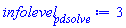
The answer to a) is now always present in the last line of the userinfo. So input infolevel[pdsolve] := 3 before calling pdsolve, and check what the last line of the userinfo displayed tells.


The answer to b) is a new option, generalsolution, implemented in pdsolve so that it either returns a general solution or otherwise it returns NULL. If you do not use this new option, then pdsolve works as always: first it tries to compute a general solution and if it fails in doing that it tries to compute a particular solution by separating the variables in different ways, or computing a traveling wave solution or etc. (a number of other well known methods).


The examples that follow are from the help page pdsolve,system, and show both the new userinfo telling whether the solution returned is a general one and the option generalsolution at work.The examples are all of differential equation systems but the same userinfos and generalsolution option work as well in the case of a single PDE.


Example 1.

Solve the determining PDE system for the infinitesimals of the symmetry generator of example 11 from Kamke's book . Tell whether the solution computed is or not a general solution.

> 

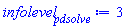
infolevel[pdsolve] := 3

3

(1.1)

The PDE system satisfied by the symmetries of Kamke's ODE example number 11 is

> 

sys__1 := [diff(xi(x, y), y, y) = 0, diff(eta(x, y), y, y)-2*(diff(xi(x, y), y, x)) = 0, 3*x^r*y^n*(diff(xi(x, y), y))*a+2*(diff(eta(x, y), y, x))-(diff(xi(x, y), x, x)) = 0, 2*(diff(xi(x, y), x))*x^r*y^n*a-x^r*y^n*(diff(eta(x, y), y))*a+eta(x, y)*a*x^r*y^n*n/y+xi(x, y)*a*x^r*r*y^n/x+diff(eta(x, y), x, x) = 0]

This is a second order linear PDE system, with two unknowns {eta(x, y), xi(x, y)} and four equations. Its general solution is given by the following, where we now can tell that the solution is a general one by reading the last line of the userinfo. Note that because the system is overdetermined, a general solution in this case does not involve any arbitrary function
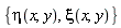
> 

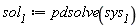
sol__1 := pdsolve(sys__1)

-> Solving ordering for the dependent variables of the PDE system: [xi(x,y), eta(x,y)]

-> Solving ordering for the independent variables (can be changed using the ivars option): [x, y]
tackling triangularized subsystem with respect to xi(x,y)
First set of solution methods (general or quasi general solution)
Trying simple case of a single derivative.
First set of solution methods successful
tackling triangularized subsystem with respect to eta(x,y)
<- Returning a *general* solution


{eta(x, y) = -_C1*y*(r+2)/(n-1), xi(x, y) = _C1*x}

(1.2)

Next we indicate to pdsolve that n and r are parameters of the problem, and that we want a solution for n <> 1, making more difficult to identify by eye whether the solution returned is or not a general one. Again the last line of the userinfo tells that pdsolve's solution is indeed a general one

> 

`sys__1.1` := [op(sys__1), n <> 1]

[diff(diff(xi(x, y), y), y) = 0, diff(diff(eta(x, y), y), y)-2*(diff(diff(xi(x, y), x), y)) = 0, 3*x^r*y^n*(diff(xi(x, y), y))*a+2*(diff(diff(eta(x, y), x), y))-(diff(diff(xi(x, y), x), x)) = 0, 2*(diff(xi(x, y), x))*x^r*y^n*a-x^r*y^n*(diff(eta(x, y), y))*a+eta(x, y)*a*x^r*y^n*n/y+xi(x, y)*a*x^r*r*y^n/x+diff(diff(eta(x, y), x), x) = 0, n <> 1]

(1.3)
> 

`sol__1.1` := pdsolve(`sys__1.1`, parameters = {n, r})

-> Solving ordering for the dependent variables of the PDE system: [r, n, xi(x,y), eta(x,y)]

-> Solving ordering for the independent variables (can be changed using the ivars option): [x, y]
tackling triangularized subsystem with respect to r
tackling triangularized subsystem with respect to n
tackling triangularized subsystem with respect to xi(x,y)
First set of solution methods (general or quasi general solution)
Trying simple case of a single derivative.
First set of solution methods successful
tackling triangularized subsystem with respect to eta(x,y)
tackling triangularized subsystem with respect to r
tackling triangularized subsystem with respect to n
tackling triangularized subsystem with respect to xi(x,y)
First set of solution methods (general or quasi general solution)
Trying simple case of a single derivative.
First set of solution methods successful
tackling triangularized subsystem with respect to eta(x,y)
tackling triangularized subsystem with respect to r
tackling triangularized subsystem with respect to n
tackling triangularized subsystem with respect to xi(x,y)
First set of solution methods (general or quasi general solution)
Trying simple case of a single derivative.
First set of solution methods successful
tackling triangularized subsystem with respect to eta(x,y)
tackling triangularized subsystem with respect to n
tackling triangularized subsystem with respect to xi(x,y)
First set of solution methods (general or quasi general solution)
Trying simple case of a single derivative.
First set of solution methods successful
tackling triangularized subsystem with respect to eta(x,y)
tackling triangularized subsystem with respect to n
tackling triangularized subsystem with respect to xi(x,y)
First set of solution methods (general or quasi general solution)
Trying simple case of a single derivative.
First set of solution methods successful
tackling triangularized subsystem with respect to eta(x,y)
tackling triangularized subsystem with respect to xi(x,y)
First set of solution methods (general or quasi general solution)
Trying simple case of a single derivative.
First set of solution methods successful
tackling triangularized subsystem with respect to eta(x,y)
<- Returning a *general* solution


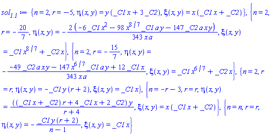
{n = 2, r = -5, eta(x, y) = y*(_C1*x+3*_C2), xi(x, y) = x*(_C1*x+_C2)}, {n = 2, r = -20/7, eta(x, y) = -(2/343)*(-6*_C1*x^2-98*x^(8/7)*_C1*a*y-147*_C2*a*x*y)/(x*a), xi(x, y) = _C1*x^(8/7)+_C2*x}, {n = 2, r = -15/7, eta(x, y) = -(1/343)*(-49*_C2*a*x*y-147*x^(6/7)*_C1*a*y+12*_C1*x)/(x*a), xi(x, y) = _C1*x^(6/7)+_C2*x}, {n = 2, r = r, eta(x, y) = -_C1*y*(r+2), xi(x, y) = _C1*x}, {n = -r-3, r = r, eta(x, y) = ((_C1*x+_C2)*r+4*_C1*x+2*_C2)*y/(r+4), xi(x, y) = x*(_C1*x+_C2)}, {n = n, r = r, eta(x, y) = -_C1*y*(r+2)/(n-1), xi(x, y) = _C1*x}

(1.4)
> 

map(pdetest, [`sol__1.1`], `sys__1.1`)

[[0, 0, 0, 0], [0, 0, 0, 0], [0, 0, 0, 0], [0, 0, 0, 0], [0, 0, 0, 0], [0, 0, 0, 0]]

(1.5)


Example 2.

Compute the solution of the following (linear) overdetermined system involving two PDEs, three unknown functions, one of which depends on 2 variables and the other two depend on only 1 variable.

> 

sys__2 := [-(diff(F(r, s), r, r))+diff(F(r, s), s, s)+diff(H(r), r)+diff(G(s), s)+s = 0, diff(F(r, s), r, r)+2*(diff(F(r, s), r, s))+diff(F(r, s), s, s)-(diff(H(r), r))+diff(G(s), s)-r = 0]

The solution for the unknowns G, H, is given by the following expression, were again determining whether this solution, that depends on 3 arbitrary functions, _F1(s), _F2(r), _F3(s-r), is or not a general solution, is non-obvious.

> 

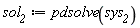
sol__2 := pdsolve(sys__2)

-> Solving ordering for the dependent variables of the PDE system: [F(r,s), H(r), G(s)]

-> Solving ordering for the independent variables (can be changed using the ivars option): [r, s]
tackling triangularized subsystem with respect to F(r,s)
First set of solution methods (general or quasi general solution)
Trying differential factorization for linear PDEs ...
differential factorization successful.
First set of solution methods successful
tackling triangularized subsystem with respect to H(r)
tackling triangularized subsystem with respect to G(s)
<- Returning a *general* solution


{F(r, s) = _F1(s)+_F2(r)+_F3(s-r)-(1/12)*r^2*(r-3*s), G(s) = -(diff(_F1(s), s))-(1/4)*s^2+_C2, H(r) = diff(_F2(r), r)-(1/4)*r^2+_C1}

(1.6)
> 

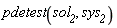
pdetest(sol__2, sys__2)

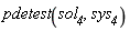
[0, 0]

(1.7)

Example 3.

Compute the solution of the following nonlinear system, consisting of Burger's equation and a possible potential.

> 

sys__3 := [diff(u(x, t), t)+2*u(x, t)*(diff(u(x, t), x))-(diff(u(x, t), x, x)) = 0, diff(v(x, t), t) = -v(x, t)*(diff(u(x, t), x))+v(x, t)*u(x, t)^2, diff(v(x, t), x) = -u(x, t)*v(x, t)]

We see that in this case the solution returned is not a general solution but two particular ones; again the information is in the last line of the userinfo displayed

> 

sol__3 := pdsolve(sys__3, [u, v])

-> Solving ordering for the dependent variables of the PDE system: [v(x,t), u(x,t)]

-> Solving ordering for the independent variables (can be changed using the ivars option): [x, t]
tackling triangularized subsystem with respect to v(x,t)
tackling triangularized subsystem with respect to u(x,t)
First set of solution methods (general or quasi general solution)
Second set of solution methods (complete solutions)
Trying methods for second order PDEs
Third set of solution methods (simple HINTs for separating variables)
PDE linear in highest derivatives - trying a separation of variables by *
HINT = *
Fourth set of solution methods
Trying methods for second order linear PDEs
Preparing a solution HINT ...
Trying HINT = _F1(x)*_F2(t)
Fourth set of solution methods
Preparing a solution HINT ...
Trying HINT = _F1(x)+_F2(t)
Trying travelling wave solutions as power series in tanh ...
* Using tau = tanh(t*C[2]+x*C[1]+C[0])
* Equivalent ODE system: {C[1]^2*(tau^2-1)^2*diff(diff(u(tau),tau),tau)+(2*C[1]^2*(tau^2-1)*tau+2*u(tau)*C[1]*(tau^2-1)+C[2]*(tau^2-1))*diff(u(tau),tau)}
* Ordering for functions: [u(tau)]
* Cases for the upper bounds: [[n[1] = 1]]
* Power series solution [1]: {u(tau) = tau*A[1,1]+A[1,0]}
* Solution [1] for {A[i, j], C[k]}: [[A[1,1] = 0], [A[1,0] = -1/2*C[2]/C[1], A[1,1] = -C[1]]]
travelling wave solutions successful.
tackling triangularized subsystem with respect to v(x,t)
First set of solution methods (general or quasi general solution)
Trying differential factorization for linear PDEs ...
Trying methods for PDEs "missing the dependent variable" ...
Second set of solution methods (complete solutions)
Trying methods for second order PDEs
Third set of solution methods (simple HINTs for separating variables)
PDE linear in highest derivatives - trying a separation of variables by *
HINT = *
Fourth set of solution methods
Trying methods for second order linear PDEs
Preparing a solution HINT ...
Trying HINT = _F1(x)*_F2(t)
Third set of solution methods successful
tackling triangularized subsystem with respect to u(x,t)
<- Returning a solution that *is not the most general one*


{u(x, t) = -_C2*tanh(_C2*x+_C3*t+_C1)-(1/2)*_C3/_C2, v(x, t) = 0}, {u(x, t) = -_c[1]^(1/2)*((exp(_c[1]^(1/2)*x))^2*_C1-_C2)/((exp(_c[1]^(1/2)*x))^2*_C1+_C2), v(x, t) = _C3*exp(_c[1]*t)*_C1*exp(_c[1]^(1/2)*x)+_C3*exp(_c[1]*t)*_C2/exp(_c[1]^(1/2)*x)}

(1.8)
> 

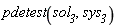
pdetest(sol__3, sys__3)

[0, 0, 0]

(1.9)

This example is also good for illustrating the other related new feature: one can now request to pdsolve to only compute a general solution (it will return NULL if it cannot achieve that). Turn OFF userinfos and try with this example

> 

infolevel[pdsolve] := 1

This returns NULL:

> 

pdsolve(sys__3, [u, v], generalsolution)

Example 4.

Another where the solution returned is particular, this time for a linear system, conformed by 38 PDEs, also from differential equation symmetry analysis

> 

sys__4 := [diff(xi[1](x, y, z, t, u), u) = 0, diff(xi[1](x, y, z, t, u), x)-(diff(xi[2](x, y, z, t, u), y)) = 0, diff(xi[2](x, y, z, t, u), u) = 0, -(diff(xi[1](x, y, z, t, u), y))-(diff(xi[2](x, y, z, t, u), x)) = 0, diff(xi[3](x, y, z, t, u), u) = 0, diff(xi[1](x, y, z, t, u), x)-(diff(xi[3](x, y, z, t, u), z)) = 0, -(diff(xi[3](x, y, z, t, u), y))-(diff(xi[2](x, y, z, t, u), z)) = 0, -(diff(xi[1](x, y, z, t, u), z))-(diff(xi[3](x, y, z, t, u), x)) = 0, diff(xi[4](x, y, z, t, u), u) = 0, diff(xi[3](x, y, z, t, u), t)-(diff(xi[4](x, y, z, t, u), z)) = 0, diff(xi[2](x, y, z, t, u), t)-(diff(xi[4](x, y, z, t, u), y)) = 0, diff(xi[1](x, y, z, t, u), t)-(diff(xi[4](x, y, z, t, u), x)) = 0, -(diff(xi[1](x, y, z, t, u), x))+diff(xi[4](x, y, z, t, u), t) = 0, diff(eta[1](x, y, z, t, u), y, y)+diff(eta[1](x, y, z, t, u), z, z)-(diff(eta[1](x, y, z, t, u), t, t))+diff(eta[1](x, y, z, t, u), x, x) = 0, diff(eta[1](x, y, z, t, u), u, u) = 0, diff(eta[1](x, y, z, t, u), u, x)+diff(xi[1](x, y, z, t, u), x, x) = 0, diff(xi[1](x, y, z, t, u), x, y)+diff(eta[1](x, y, z, t, u), u, y) = 0, -(diff(xi[1](x, y, z, t, u), y, y))+diff(eta[1](x, y, z, t, u), u, x) = 0, diff(xi[1](x, y, z, t, u), x, z)+diff(eta[1](x, y, z, t, u), u, z) = 0, diff(xi[1](x, y, z, t, u), y, z) = 0, -(diff(xi[1](x, y, z, t, u), z, z))+diff(eta[1](x, y, z, t, u), u, x) = 0, -(diff(eta[1](x, y, z, t, u), t, u))-(diff(xi[1](x, y, z, t, u), t, x)) = 0, diff(xi[1](x, y, z, t, u), t, y) = 0, diff(xi[1](x, y, z, t, u), t, z) = 0, diff(xi[1](x, y, z, t, u), t, t)+diff(eta[1](x, y, z, t, u), u, x) = 0, -(diff(xi[2](x, y, z, t, u), z, z))+diff(eta[1](x, y, z, t, u), u, y) = 0, diff(xi[2](x, y, z, t, u), t, z) = 0, diff(xi[2](x, y, z, t, u), t, t)+diff(eta[1](x, y, z, t, u), u, y) = 0, diff(xi[3](x, y, z, t, u), t, t)+diff(eta[1](x, y, z, t, u), u, z) = 0, diff(eta[1](x, y, z, t, u), u, x, x) = 0, diff(eta[1](x, y, z, t, u), u, x, y) = 0, diff(eta[1](x, y, z, t, u), u, y, y) = 0, diff(eta[1](x, y, z, t, u), u, x, z) = 0, diff(eta[1](x, y, z, t, u), u, y, z) = 0, diff(eta[1](x, y, z, t, u), u, z, z) = 0, diff(eta[1](x, y, z, t, u), t, u, x) = 0, diff(eta[1](x, y, z, t, u), t, u, y) = 0, diff(eta[1](x, y, z, t, u), t, u, z) = 0]

There are 38 coupled equations

> 

nops(sys__4)

38

(1.10)

When requesting a general solution pdsolve returns NULL:

> 

pdsolve(sys__4, generalsolution)

A solution that is not a general one, is however computed by default if calling pdsolve without the generalsolution option. In this case again the last line of the userinfo tells that the solution returned is not a general solution

> 

infolevel[pdsolve] := 3

3

(1.11)
> 

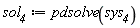
sol__4 := pdsolve(sys__4)

-> Solving ordering for the dependent variables of the PDE system: [eta[1](x,y,z,t,u), xi[1](x,y,z,t,u), xi[2](x,y,z,t,u), xi[3](x,y,z,t,u), xi[4](x,y,z,t,u)]

-> Solving ordering for the independent variables (can be changed using the ivars option): [t, x, y, z, u]
tackling triangularized subsystem with respect to eta[1](x,y,z,t,u)
First set of solution methods (general or quasi general solution)
Trying simple case of a single derivative.
First set of solution methods successful
-> Solving ordering for the dependent variables of the PDE system: [_F1(x,y,z,t), _F2(x,y,z,t)]
-> Solving ordering for the independent variables (can be changed using the ivars option): [t, x, y, z, u]
tackling triangularized subsystem with respect to _F1(x,y,z,t)
First set of solution methods (general or quasi general solution)
Trying simple case of a single derivative.
First set of solution methods successful
-> Solving ordering for the dependent variables of the PDE system: [_F3(x,y,z), _F4(x,y,z)]
-> Solving ordering for the independent variables (can be changed using the ivars option): [x, y, z, t]
tackling triangularized subsystem with respect to _F3(x,y,z)
First set of solution methods (general or quasi general solution)
Trying simple case of a single derivative.
First set of solution methods successful
First set of solution methods (general or quasi general solution)
Trying simple case of a single derivative.
First set of solution methods successful
tackling triangularized subsystem with respect to _F4(x,y,z)
First set of solution methods (general or quasi general solution)
Trying simple case of a single derivative.
First set of solution methods successful
-> Solving ordering for the dependent variables of the PDE system: [_F5(y,z), _F6(y,z)]
-> Solving ordering for the independent variables (can be changed using the ivars option): [y, z, x]
tackling triangularized subsystem with respect to _F5(y,z)
First set of solution methods (general or quasi general solution)
Trying simple case of a single derivative.
First set of solution methods successful
tackling triangularized subsystem with respect to _F6(y,z)
First set of solution methods (general or quasi general solution)
Trying simple case of a single derivative.
First set of solution methods successful
-> Solving ordering for the dependent variables of the PDE system: [_F7(z), _F8(z)]
-> Solving ordering for the independent variables (can be changed using the ivars option): [z, y]
tackling triangularized subsystem with respect to _F7(z)
tackling triangularized subsystem with respect to _F8(z)
tackling triangularized subsystem with respect to _F2(x,y,z,t)
First set of solution methods (general or quasi general solution)
Trying differential factorization for linear PDEs ...
Trying methods for PDEs "missing the dependent variable" ...
Second set of solution methods (complete solutions)
Third set of solution methods (simple HINTs for separating variables)
PDE linear in highest derivatives - trying a separation of variables by *
HINT = *
Fourth set of solution methods
Preparing a solution HINT ...
Trying HINT = _F3(x)*_F4(y)*_F5(z)*_F6(t)
Third set of solution methods successful

tackling triangularized subsystem with respect to xi[1](x,y,z,t,u)
First set of solution methods (general or quasi general solution)
Trying simple case of a single derivative.
First set of solution methods successful
First set of solution methods (general or quasi general solution)
Trying simple case of a single derivative.
First set of solution methods successful
-> Solving ordering for the dependent variables of the PDE system: [_F1(x,z,t), _F2(x,z,t)]
-> Solving ordering for the independent variables (can be changed using the ivars option): [t, x, z, y]
tackling triangularized subsystem with respect to _F1(x,z,t)
First set of solution methods (general or quasi general solution)
Trying simple case of a single derivative.
First set of solution methods successful
First set of solution methods (general or quasi general solution)
Trying simple case of a single derivative.
First set of solution methods successful
tackling triangularized subsystem with respect to _F2(x,z,t)
First set of solution methods (general or quasi general solution)
Trying simple case of a single derivative.
First set of solution methods successful

-> Solving ordering for the dependent variables of the PDE system: [_F3(x,t), _F4(x,t)]
-> Solving ordering for the independent variables (can be changed using the ivars option): [t, x, z]
tackling triangularized subsystem with respect to _F3(x,t)
First set of solution methods (general or quasi general solution)
Trying simple case of a single derivative.
First set of solution methods successful
tackling triangularized subsystem with respect to _F4(x,t)
First set of solution methods (general or quasi general solution)
Trying simple case of a single derivative.
First set of solution methods successful
-> Solving ordering for the dependent variables of the PDE system: [_F5(x), _F6(x)]
-> Solving ordering for the independent variables (can be changed using the ivars option): [x, t]
tackling triangularized subsystem with respect to _F5(x)
tackling triangularized subsystem with respect to _F6(x)
tackling triangularized subsystem with respect to xi[2](x,y,z,t,u)
First set of solution methods (general or quasi general solution)
Trying simple case of a single derivative.
First set of solution methods successful
First set of solution methods (general or quasi general solution)
Trying simple case of a single derivative.
First set of solution methods successful
First set of solution methods (general or quasi general solution)
Trying simple case of a single derivative.
First set of solution methods successful
First set of solution methods (general or quasi general solution)
Trying simple case of a single derivative.
First set of solution methods successful
-> Solving ordering for the dependent variables of the PDE system: [_F1(t), _F2(t)]
-> Solving ordering for the independent variables (can be changed using the ivars option): [t, z]
tackling triangularized subsystem with respect to _F1(t)
tackling triangularized subsystem with respect to _F2(t)
tackling triangularized subsystem with respect to xi[3](x,y,z,t,u)
First set of solution methods (general or quasi general solution)
Trying simple case of a single derivative.
First set of solution methods successful
First set of solution methods (general or quasi general solution)
Trying simple case of a single derivative.
First set of solution methods successful
First set of solution methods (general or quasi general solution)
Trying simple case of a single derivative.
First set of solution methods successful
First set of solution methods (general or quasi general solution)
Trying simple case of a single derivative.
First set of solution methods successful
tackling triangularized subsystem with respect to xi[4](x,y,z,t,u)
First set of solution methods (general or quasi general solution)
Trying simple case of a single derivative.
First set of solution methods successful
First set of solution methods (general or quasi general solution)
Trying simple case of a single derivative.
First set of solution methods successful
First set of solution methods (general or quasi general solution)
Trying simple case of a single derivative.
First set of solution methods successful
First set of solution methods (general or quasi general solution)
Trying simple case of a single derivative.
First set of solution methods successful
<- Returning a solution that *is not the most general one*


{eta[1](x, y, z, t, u) = (_C13*(_C10*(exp(_c[3]^(1/2)*z))^2+_C11)*(_C8*(exp(_c[2]^(1/2)*y))^2+_C9)*(_C6*(exp(_c[1]^(1/2)*x))^2+_C7)*cos((-_c[1]-_c[2]-_c[3])^(1/2)*t)+_C12*(_C10*(exp(_c[3]^(1/2)*z))^2+_C11)*(_C8*(exp(_c[2]^(1/2)*y))^2+_C9)*(_C6*(exp(_c[1]^(1/2)*x))^2+_C7)*sin((-_c[1]-_c[2]-_c[3])^(1/2)*t)+u*exp(_c[1]^(1/2)*x)*exp(_c[2]^(1/2)*y)*exp(_c[3]^(1/2)*z)*(_C1*t+_C2*x+_C3*y+_C4*z+_C5))/(exp(_c[1]^(1/2)*x)*exp(_c[2]^(1/2)*y)*exp(_c[3]^(1/2)*z)), xi[1](x, y, z, t, u) = -(1/2)*_C2*x^2+(1/2)*(-2*_C1*t-2*_C3*y-2*_C4*z+2*_C17)*x+(1/2)*(-t^2+y^2+z^2)*_C2+_C16*t+_C15*z+_C14*y+_C18, xi[2](x, y, z, t, u) = -(1/2)*_C3*y^2+(1/2)*(-2*_C1*t-2*_C2*x-2*_C4*z+2*_C17)*y+(1/2)*(-t^2+x^2+z^2)*_C3+_C20*t+_C19*z-_C14*x+_C21, xi[3](x, y, z, t, u) = -(1/2)*_C4*z^2+(1/2)*(-2*_C1*t-2*_C2*x-2*_C3*y+2*_C17)*z+(1/2)*(-t^2+x^2+y^2)*_C4+_C22*t-_C19*y-_C15*x+_C23, xi[4](x, y, z, t, u) = -(1/2)*_C1*t^2+(1/2)*(-2*_C2*x-2*_C3*y-2*_C4*z+2*_C17)*t+(1/2)*(-x^2-y^2-z^2)*_C1+_C20*y+_C22*z+_C16*x+_C24}

(1.12)
> 

pdetest(sol__4, sys__4)

[0, 0, 0, 0, 0, 0, 0, 0, 0, 0, 0, 0, 0, 0, 0, 0, 0, 0, 0, 0, 0, 0, 0, 0, 0, 0, 0, 0, 0, 0, 0, 0, 0, 0, 0, 0, 0, 0]

(1.13)

Example 5.

Finally, the new userinfos also tell whether a solution is or not a general solution when working with PDEs that involve anticommutative variables  set using the Physics  package

> 

with(Physics, Setup)

[Setup]

(1.14)

Set first theta and Q as suffixes for variables of type/anticommutative  (see Setup )

> 

Setup(anticommutativepre = {Q, theta})

`* Partial match of  'anticommutativepre' against keyword 'anticommutativeprefix'`


[anticommutativeprefix = {Q, _lambda, theta}]

(1.15)

A PDE system example with two unknown anticommutative functions of four variables, two commutative and two anticommutative; to avoid redundant typing in the input that follows and redundant display of information on the screen let's use PDEtools:-diff_table   PDEtools:-declare

> 

PDEtools:-declare(Q(x, y, theta[1], theta[2]))

Q(x, y, theta[1], theta[2])*`will now be displayed as`*Q

(1.16)
> 

q := PDEtools:-diff_table(Q(x, y, theta[1], theta[2]))

table( [(  ) = Q(x, y, theta[1], theta[2]) ] )

(1.17)

Consider the system formed by these two PDEs (because of the q diff_table just defined, we can enter derivatives directly using the function's name indexed by the differentiation variables)

> 

pde[1] := q[x, y, theta[1]]+q[x, y, theta[2]]-q[y, theta[1], theta[2]] = 0

Physics:-diff(diff(diff(Q(x, y, theta[1], theta[2]), x), y), theta[1])+Physics:-diff(diff(diff(Q(x, y, theta[1], theta[2]), x), y), theta[2])-Physics:-diff(Physics:-diff(diff(Q(x, y, theta[1], theta[2]), y), theta[1]), theta[2]) = 0

(1.18)
> 

pde[2] := q[theta[1]] = 0

Physics:-diff(Q(x, y, theta[1], theta[2]), theta[1]) = 0

(1.19)

The solution returned for this system is indeed a general solution

> 

pdsolve([pde[1], pde[2]])

-> Solving ordering for the dependent variables of the PDE system: [_F4(x,y), _F2(x,y), _F3(x,y)]

-> Solving ordering for the independent variables (can be changed using the ivars option): [x, y]
tackling triangularized subsystem with respect to _F4(x,y)
tackling triangularized subsystem with respect to _F2(x,y)
tackling triangularized subsystem with respect to _F3(x,y)
First set of solution methods (general or quasi general solution)
Trying simple case of a single derivative.
HINT = _F6(x)+_F5(y)
Trying HINT = _F6(x)+_F5(y)
HINT is successful
First set of solution methods successful
<- Returning a *general* solution


Q(x, y, theta[1], theta[2]) = _F1(x, y)*_lambda1+(_F6(x)+_F5(y))*theta[2]

(1.20)
> 

NULL

This solution involves an anticommutative constant `_&lambda;2`, analogous to the commutative constants _Cn where n is an integer.


Download PDE_general_solutions.mw

Edgardo S. Cheb-Terrab
Physics, Differential Equations and Mathematical Functions, Maplesoft


Hi

New developments (after the release of Maple 2016) happened in the project on exact solutions for "Partial Differential Equations & Boundary Conditions". This is work in collaboration with Katherina von Bulow and the improvements are of wide range, representing a noticeable step forward in the capabilities of the Maple system for this kind of problem. As usual, these improvements can be installed in current Maple 2016 by downloading the updated library from the Maplesoft R&D webpage for Differential Equations and Mathematical functions (the update is distributed merged with the updates of the Physics package)


The improvements cover:


• 

PDE&BC in semi-infinite domains for which a bounded solution is sought

• 

PDE & BC problems in bounded spatial domains via eigenfunction (Fourier) expansions

• 

Implementation of another algebraic method for tackling linear PDE & BC

• 

Improvements in solving PDE & BC solutions by first finding the PDE's general solution.

• 

Improvements in solving PDE & BC problems by using a Fourier transform.

• 

PDE & BC problems that used to require the option HINT = `+` are now solved automatically


What follows is a set of examples solved now with these new developments, organized in sections according to the kind of problem. Where relevant, the sections include a subsection on "How it works step by step".

PDE&BC in semi-infinite domains for which a bounded solution is sought can now also be solved via Laplace transforms


Maple is now able to solve more PDE&BC problems via Laplace transforms.


How it works: Laplace transforms act to change derivatives with respect to one of the independent variables of the domain into multiplication operations in the transformed domain. After applying a Laplace transform to the original problem, we can simplify the problem using the transformed BC, then solve the problem in the transformed domain, and finally apply the inverse Laplace transform to arrive at the final solution. It is important to remember to give pdsolve any necessary restrictions on the variables and constants of the problem, by means of the "assuming" command.


A new feature is that we can now tell pdsolve that the dependent variable is bounded, by means of the optional argument HINT = boundedseries.


> 

restart


Consider the problem of a falling cable lying on a table that is suddenly removed (cf. David J. Logan's Applied Partial Differential Equations p.115).

> 

pde[1] := diff(u(x, t), t, t) = c^2*(diff(u(x, t), x, x))-g
iv[1] := u(x, 0) = 0, u(0, t) = 0, (D[2](u))(x, 0) = 0


If we ask pdsolve to solve this problem without the condition of boundedness of the solution, we obtain:

> 

`assuming`([pdsolve([pde[1], iv[1]])], [0 < t, 0 < x, 0 < c])

u(x, t) = -invlaplace(exp(s*x/c)*_F1(s), s, t)+invlaplace(exp(-s*x/c)*_F1(s), s, t)-(1/2)*g*t^2+invlaplace(exp(s*x/c)/s^3, s, t)*g

(1.1)

New: If we now ask for a bounded solution, by means of the option HINT = boundedseries, pdsolve simplifies the problem accordingly.

> 

ans[1] := `assuming`([pdsolve([pde[1], iv[1]], HINT = boundedseries)], [0 < t, 0 < x, 0 < c])

u(x, t) = (1/2)*g*(Heaviside(t-x/c)*(c*t-x)^2-c^2*t^2)/c^2

(1.2)


And we can check this answer against the original problem, if desired:

> 

`assuming`([pdetest(ans[1], [pde[1], iv[1]])], [0 < t, 0 < x, 0 < c])

[0, 0, 0, 0]

(1.3)

How it works, step by step


 Let us see the process this problem undergoes to be solved by pdsolve, step by step.


First, the Laplace transform is applied to the PDE:

> 

with(inttrans)

> 

transformed_PDE := laplace((lhs-rhs)(pde[1]), t, s)

s^2*laplace(u(x, t), t, s)-(D[2](u))(x, 0)-s*u(x, 0)-c^2*(diff(diff(laplace(u(x, t), t, s), x), x))+g/s

(1.1.1)

and the result is simplified using the initial conditions:

> 

simplified_transformed_PDE := eval(transformed_PDE, {iv[1]})

s^2*laplace(u(x, t), t, s)-c^2*(diff(diff(laplace(u(x, t), t, s), x), x))+g/s

(1.1.2)

Next, we call the function "laplace(u(x,t),t,s)" by the new name U:

> 

eq_U := subs(laplace(u(x, t), t, s) = U(x, s), simplified_transformed_PDE)

s^2*U(x, s)-c^2*(diff(diff(U(x, s), x), x))+g/s

(1.1.3)

And this equation, which is really an ODE, is solved:

> 

solution_U := dsolve(eq_U, U(x, s))

U(x, s) = exp(-s*x/c)*_F2(s)+exp(s*x/c)*_F1(s)-g/s^3

(1.1.4)

Now, since we want a BOUNDED solution, the term with the positive exponential must be zero, and we are left with:

> 

bounded_solution_U := subs(coeff(rhs(solution_U), exp(s*x/c)) = 0, solution_U)

U(x, s) = exp(-s*x/c)*_F2(s)-g/s^3

(1.1.5)

Now, the initial solution must also be satisfied. Here it is, in the transformed domain:

> 

Laplace_BC := laplace(u(0, t), t, s) = 0

laplace(u(0, t), t, s) = 0

(1.1.6)

Or, in the new variable U,

> 

Laplace_BC_U := U(0, s) = 0

U(0, s) = 0

(1.1.7)

And by applying it to bounded_solution_U, we find the relationship

> 

simplify(subs(x = 0, rhs(bounded_solution_U))) = 0

(_F2(s)*s^3-g)/s^3 = 0

(1.1.8)
> 

isolate((_F2(s)*s^3-g)/s^3 = 0, indets((_F2(s)*s^3-g)/s^3 = 0, unknown)[1])

_F2(s) = g/s^3

(1.1.9)

so that our solution now becomes

> 

bounded_solution_U := subs(_F2(s) = g/s^3, bounded_solution_U)

U(x, s) = exp(-s*x/c)*g/s^3-g/s^3

(1.1.10)

to which we now apply the inverse Laplace transform to obtain the solution to the problem:

> 

`assuming`([u(x, t) = invlaplace(rhs(bounded_solution_U), s, t)], [0 < x, 0 < t, 0 < c])

u(x, t) = (1/2)*g*(-t^2+Heaviside(t-x/c)*(c*t-x)^2/c^2)

(1.1.11)

Four other related examples


A few other examples:

> 

pde[2] := diff(u(x, t), t, t) = c^2*(diff(u(x, t), x, x))
iv[2] := u(x, 0) = 0, u(0, t) = g(t), (D[2](u))(x, 0) = 0

> 

ans[2] := `assuming`([pdsolve([pde[2], iv[2]], HINT = boundedseries)], [0 < t, 0 < x, 0 < c])

u(x, t) = Heaviside(t-x/c)*g((c*t-x)/c)

(1.2.1)
> 

`assuming`([pdetest(ans[2], [pde[2], iv[2]])], [0 < t, 0 < x, 0 < c])

[0, 0, 0, 0]

(1.2.2)
> 

pde[3] := diff(u(x, t), t) = k*(diff(u(x, t), x, x)); iv[3] := u(x, 0) = 0, u(0, t) = 1

> 

ans[3] := `assuming`([pdsolve([pde[3], iv[3]], HINT = boundedseries)], [0 < t, 0 < x, 0 < k])

u(x, t) = 1-erf((1/2)*x/(t^(1/2)*k^(1/2)))

(1.2.3)
> 

pdetest(ans[3], [pde[3], iv[3][2]])

[0, 0]

(1.2.4)
> 

pde[4] := diff(u(x, t), t) = k*(diff(u(x, t), x, x)); iv[4] := u(x, 0) = mu, u(0, t) = lambda

> 

ans[4] := `assuming`([pdsolve([pde[4], iv[4]], HINT = boundedseries)], [0 < t, 0 < x, 0 < k])

u(x, t) = (-lambda+mu)*erf((1/2)*x/(t^(1/2)*k^(1/2)))+lambda

(1.2.5)
> 

pdetest(ans[4], [pde[4], iv[4][2]])

[0, 0]

(1.2.6)


The following is an example from page 76 in Logan's book:

> 

pde[5] := diff(u(x, t), t) = diff(u(x, t), x, x)
iv[5] := u(x, 0) = 0, u(0, t) = f(t)

> 

ans[5] := `assuming`([pdsolve([pde[5], iv[5]], HINT = boundedseries)], [0 < t, 0 < x])

u(x, t) = (1/2)*x*(int(f(_U1)*exp(-x^2/(4*t-4*_U1))/(t-_U1)^(3/2), _U1 = 0 .. t))/Pi^(1/2)

(1.2.7)

More PDE&BC problems in bounded spatial domains can now be solved via eigenfunction (Fourier) expansions


The code for solving PDE&BC problems in bounded spatial domains has been expanded. The method works by separating the variables by product, so that the problem is transformed into an ODE system (with initial and/or boundary conditions) problem, one of which is a Sturm-Liouville problem (a type of eigenvalue problem) which has infinitely many solutions - hence the infinite series representation of the solutions.

> 

restart


Here is a simple example for the heat equation:

> 

pde__6 := diff(u(x, t), t) = k*(diff(u(x, t), x, x)); iv__6 := u(0, t) = 0, u(l, t) = 0

> 

ans__6 := `assuming`([pdsolve([pde__6, iv__6])], [0 < l])

u(x, t) = Sum(_C1*sin(_Z1*Pi*x/l)*exp(-k*Pi^2*_Z1^2*t/l^2), _Z1 = 1 .. infinity)

(2.1)
> 

pdetest(ans__6, [pde__6, iv__6])

[0, 0, 0]

(2.2)


Now, consider the displacements of a string governed by the wave equation, where c is a constant (cf. Logan p.28).

> 

pde__7 := diff(u(x, t), t, t) = c^2*(diff(u(x, t), x, x))
iv__7 := u(0, t) = 0, u(l, t) = 0

> 

ans__7 := `assuming`([pdsolve([pde__7, iv__7])], [0 < l])

u(x, t) = Sum(sin(_Z2*Pi*x/l)*(sin(c*_Z2*Pi*t/l)*_C1+cos(c*_Z2*Pi*t/l)*_C5), _Z2 = 1 .. infinity)

(2.3)
> 

pdetest(ans__7, [pde__7, iv__7])

[0, 0, 0]

(2.4)

Another wave equation problem (cf. Logan p.130):

> 

pde__8 := diff(u(x, t), t, t)-c^2*(diff(u(x, t), x, x)) = 0; iv__8 := u(0, t) = 0, (D[2](u))(x, 0) = 0, (D[1](u))(l, t) = 0, u(x, 0) = f(x)

> 

ans__8 := `assuming`([pdsolve([pde__8, iv__8], u(x, t))], [0 <= x, x <= l])

u(x, t) = Sum(2*(Int(f(x)*sin((1/2)*Pi*(2*_Z3+1)*x/l), x = 0 .. l))*sin((1/2)*Pi*(2*_Z3+1)*x/l)*cos((1/2)*c*Pi*(2*_Z3+1)*t/l)/l, _Z3 = 1 .. infinity)

(2.5)
> 

pdetest(ans__8, [pde__8, iv__8[1 .. 3]])

[0, 0, 0, 0]

(2.6)


Here is a problem with periodic boundary conditions (cf. Logan p.131). The function u(x, t) stands for the concentration of a chemical dissolved in water within a tubular ring of circumference 2*l. The initial concentration is given by f(x), and the variable x is the arc-length parameter that varies from 0 to 2*l.

> 

pde__9 := diff(u(x, t), t) = M*(diff(u(x, t), x, x))
iv__9 := u(0, t) = u(2*l, t), (D[1](u))(0, t) = (D[1](u))(2*l, t), u(x, 0) = f(x)

> 

ans__9 := `assuming`([pdsolve([pde__9, iv__9], u(x, t))], [0 <= x, x <= 2*l])

u(x, t) = (1/2)*_C8+Sum(((Int(f(x)*sin(_Z4*Pi*x/l), x = 0 .. 2*l))*sin(_Z4*Pi*x/l)+(Int(f(x)*cos(_Z4*Pi*x/l), x = 0 .. 2*l))*cos(_Z4*Pi*x/l))*exp(-M*Pi^2*_Z4^2*t/l^2)/l, _Z4 = 1 .. infinity)

(2.7)
> 

pdetest(ans__9, [pde__9, iv__9[1 .. 2]])

[0, 0, 0]

(2.8)


The following problem is for heat flow with both boundaries insulated (cf. Logan p.166, 3rd edition)

> 

pde__10 := diff(u(x, t), t) = k*(diff(u(x, t), x, x))
iv__10 := (D[1](u))(0, t) = 0, (D[1](u))(l, t) = 0, u(x, 0) = f(x)

> 

ans__10 := `assuming`([pdsolve([pde__10, iv__10], u(x, t))], [0 <= x, x <= l])

u(x, t) = Sum(2*(Int(f(x)*cos(_Z6*Pi*x/l), x = 0 .. l))*cos(_Z6*Pi*x/l)*exp(-k*Pi^2*_Z6^2*t/l^2)/l, _Z6 = 1 .. infinity)

(2.9)
> 

pdetest(ans__10, [pde__10, iv__10[1 .. 2]])

[0, 0, 0]

(2.10)


This is a problem in a bounded domain with the presence of a source. A source term represents an outside influence in the system and leads to an inhomogeneous PDE (cf. Logan p.149):

> 

pde__11 := diff(u(x, t), t, t)-c^2*(diff(u(x, t), x, x)) = p(x, t)
iv__11 := u(0, t) = 0, u(Pi, t) = 0, u(x, 0) = 0, (D[2](u))(x, 0) = 0

> 

ans__11 := pdsolve([pde__11, iv__11], u(x, t))

u(x, t) = Int(Sum(2*(Int(p(x, tau1)*sin(_Z7*x), x = 0 .. Pi))*sin(_Z7*x)*sin(c*_Z7*(t-tau1))/(Pi*_Z7*c), _Z7 = 1 .. infinity), tau1 = 0 .. t)

(2.11)

Current pdetest is unable to verify that this solution cancells the pde__11 mainly because it currently fails in identifying that there is a fourier expansion in it, but its subroutines for testing the boundary conditions work well with this problem

> 

pdetest_BC := `pdetest/BC`

> 

pdetest_BC({ans__11}, [iv__11], [u(x, t)])

[0, 0, 0, 0]

(2.12)


Consider a heat absorption-radiation problem in the bounded domain 0 <= x and x <= 2, t >= 0:

> 

pde__12 := diff(u(x, t), t) = diff(u(x, t), x, x)
iv__12 := u(x, 0) = f(x), (D[1](u))(0, t)+u(0, t) = 0, (D[1](u))(2, t)+u(2, t) = 0

> 

ans__12 := `assuming`([pdsolve([pde__12, iv__12], u(x, t))], [0 <= x and x <= 2, 0 <= t])

u(x, t) = (1/2)*_C8+Sum(((Int(f(x)*cos((1/2)*_Z8*Pi*x), x = 0 .. 2))*cos((1/2)*_Z8*Pi*x)+(Int(f(x)*sin((1/2)*_Z8*Pi*x), x = 0 .. 2))*sin((1/2)*_Z8*Pi*x))*exp(-(1/4)*Pi^2*_Z8^2*t), _Z8 = 1 .. infinity)

(2.13)
> 

pdetest(ans__12, pde__12)

0

(2.14)

Consider the nonhomogeneous wave equation problem (cf. Logan p.213, 3rd edition):

> 

pde__13 := diff(u(x, t), t, t) = A*x+diff(u(x, t), x, x)
iv__13 := u(0, t) = 0, u(1, t) = 0, u(x, 0) = 0, (D[2](u))(x, 0) = 0

> 

ans__13 := pdsolve([pde__13, iv__13])

u(x, t) = Int(Sum(2*A*(Int(x*sin(Pi*_Z9*x), x = 0 .. 1))*sin(Pi*_Z9*x)*sin(Pi*_Z9*(t-tau1))/(Pi*_Z9), _Z9 = 1 .. infinity), tau1 = 0 .. t)

(2.15)
> 

pdetest_BC({ans__13}, [iv__13], [u(x, t)])

[0, 0, 0, 0]

(2.16)


Consider the following Schrödinger equation with zero potential energy (cf. Logan p.30):

> 

pde__14 := I*h*(diff(f(x, t), t)) = -h^2*(diff(f(x, t), x, x))/(2*m)
iv__14 := f(0, t) = 0, f(d, t) = 0

> 

ans__14 := `assuming`([pdsolve([pde__14, iv__14])], [0 < d])

f(x, t) = Sum(_C1*sin(_Z10*Pi*x/d)*exp(-((1/2)*I)*h*Pi^2*_Z10^2*t/(d^2*m)), _Z10 = 1 .. infinity)

(2.17)
> 

pdetest(ans__14, [pde__14, iv__14])

[0, 0, 0]

(2.18)

Another method has been implemented for linear PDE&BC


This method is for problems of the form


 "(&PartialD;w)/(&PartialD;t)=M[w]"", w(`x__i`,0) = f(`x__i`)" or


"((&PartialD;)^2w)/((&PartialD;)^( )t^2)="M[w]", w(`x__i`,0) = f(`x__i`), (&PartialD;w)/(&PartialD;t)() ? ()|() ? (t=0) =g(`x__i`)"


where M is an arbitrary linear differential operator of any order which only depends on the spatial variables x__i.


Here are some examples:

> 

pde__15 := diff(w(x1, x2, x3, t), t)-(diff(w(x1, x2, x3, t), x2, x1))-(diff(w(x1, x2, x3, t), x3, x1))-(diff(w(x1, x2, x3, t), x3, x3))+diff(w(x1, x2, x3, t), x3, x2) = 0
iv__15 := w(x1, x2, x3, 0) = x1^5*x2*x3NULL

> 

pdsolve([pde__15, iv__15])

w(x1, x2, x3, t) = 20*(((1/20)*x2*x3-(1/20)*t)*x1^2+(1/4)*t*(x2+x3)*x1+t^2)*x1^3

(3.1)
> 

pdetest(%, [pde__15, iv__15])

[0, 0]

(3.2)


Here are two examples for which the derivative with respect to t is of the second order, and two initial conditions are given:

> 

pde__16 := diff(w(x1, x2, x3, t), t, t) = diff(w(x1, x2, x3, t), x2, x1)+diff(w(x1, x2, x3, t), x3, x1)+diff(w(x1, x2, x3, t), x3, x3)-(diff(w(x1, x2, x3, t), x3, x2))
iv__16 := w(x1, x2, x3, 0) = x1^3*x2^2+x3, (D[4](w))(x1, x2, x3, 0) = -x2*x3+x1

> 

pdsolve([pde__16, iv__16])

w(x1, x2, x3, t) = x1^3*x2^2+x3-t*x2*x3+t*x1+3*t^2*x2*x1^2+(1/6)*t^3+(1/2)*t^4*x1

(3.3)
> 

pdetest(%, [pde__16, iv__16])

[0, 0, 0]

(3.4)
> 

pde__17 := diff(w(x1, x2, x3, t), t, t) = diff(w(x1, x2, x3, t), x2, x1)+diff(w(x1, x2, x3, t), x3, x1)+diff(w(x1, x2, x3, t), x3, x3)-(diff(w(x1, x2, x3, t), x3, x2))
iv__17 := w(x1, x2, x3, 0) = x1^3*x3^2+sin(x1), (D[4](w))(x1, x2, x3, 0) = cos(x1)-x2*x3

> 

pdsolve([pde__17, iv__17])

w(x1, x2, x3, t) = (1/2)*t^4*x1+t^2*x1^3+3*t^2*x1^2*x3+x1^3*x3^2+(1/6)*t^3-t*x2*x3+cos(x1)*t+sin(x1)

(3.5)
> 

pdetest(%, [pde__17, iv__17])

[0, 0, 0]

(3.6)

More PDE&BC problems are now solved via first finding the PDE's general solution.


The following are examples of PDE&BC problems for which pdsolve is successful in first calculating the PDE's general solution, and then fitting the initial or boundary condition to it.

> 

pde__18 := diff(u(x, y), x, x)+diff(u(x, y), y, y) = 0
iv__18 := u(0, y) = sin(y)/y

If we ask pdsolve to solve the problem, we get:

> 

ans__18 := pdsolve([pde__18, iv__18])

u(x, y) = (sin(-y+I*x)+_F2(y-I*x)*(y-I*x)+(-y+I*x)*_F2(y+I*x))/(-y+I*x)

(4.1)

and we can check this answer by using pdetest:

> 

pdetest(ans__18, [pde__18, iv__18])

[0, 0]

(4.2)

How it works, step by step:


The general solution for just the PDE is:

> 

gensol := pdsolve(pde__18)

u(x, y) = _F1(y-I*x)+_F2(y+I*x)

(4.1.1)

Substituting in the condition iv__18, we get:

u(0, y) = sin(y)/y

(4.1.2)
> 

gensol_with_condition := eval(rhs(gensol), x = 0) = rhs(iv__18)

_F1(y)+_F2(y) = sin(y)/y

(4.1.3)

We then isolate one of the functions above (we can choose either one, in this case), convert it into a function operator, and then apply it to gensol

> 

_F1 = unapply(solve(_F1(y)+_F2(y) = sin(y)/y, _F1(y)), y)

_F1 = (proc (y) options operator, arrow; (-_F2(y)*y+sin(y))/y end proc)

(4.1.4)
> 

eval(gensol, _F1 = (proc (y) options operator, arrow; (-_F2(y)*y+sin(y))/y end proc))

u(x, y) = (-_F2(y-I*x)*(y-I*x)-sin(-y+I*x))/(y-I*x)+_F2(y+I*x)

(4.1.5)


Three other related examples

 
> 

pde__19 := diff(u(x, y), x, x)+(1/2)*(diff(u(x, y), y, y)) = 0
iv__19 := u(0, y) = sin(y)/y

> 

pdsolve([pde__19, iv__19])

u(x, y) = (2*sin(-y+((1/2)*I)*2^(1/2)*x)+(-I*2^(1/2)*x+2*y)*_F2(y-((1/2)*I)*2^(1/2)*x)+(I*2^(1/2)*x-2*y)*_F2(y+((1/2)*I)*2^(1/2)*x))/(I*2^(1/2)*x-2*y)

(4.2.1)
> 

pdetest(%, [pde__19, iv__19])

[0, 0]

(4.2.2)
> 

pde__20 := diff(u(x, y), x, x)+(1/2)*(diff(u(x, y), y, y)) = 0
iv__20 := u(x, 0) = sin(x)/x

> 

pdsolve([pde__20, iv__20])

u(x, y) = (sinh((1/2)*(I*2^(1/2)*x-2*y)*2^(1/2))*2^(1/2)-(I*2^(1/2)*x-2*y)*(_F2(-y+((1/2)*I)*2^(1/2)*x)-_F2(y+((1/2)*I)*2^(1/2)*x)))/(I*2^(1/2)*x-2*y)

(4.2.3)
> 

pdetest(%, [pde__20, iv__20])

[0, 0]

(4.2.4)
> 

pde__21 := diff(u(r, t), r, r)+(diff(u(r, t), r))/r+(diff(u(r, t), t, t))/r^2 = 0
iv__21 := u(3, t) = sin(6*t)

> 

ans__21 := pdsolve([pde__21, iv__21])

u(r, t) = -_F2(-(2*I)*ln(3)+I*ln(r)+t)+sin(-(6*I)*ln(3)+(6*I)*ln(r)+6*t)+_F2(-I*ln(r)+t)

(4.2.5)
> 

pdetest(ans__21, [pde__21, iv__21])

[0, 0]

(4.2.6)

More PDE&BC problems are now solved by using a Fourier transform.

 
> 

restart

Consider the following problem with an initial condition:

> 

pde__22 := diff(u(x, t), t) = diff(u(x, t), x, x)+m
iv__22 := u(x, 0) = sin(x)


pdsolve can solve this problem directly:

> 

ans__22 := pdsolve([pde__22, iv__22])

u(x, t) = sin(x)*exp(-t)+m*t

(5.1)

And we can check this answer against the original problem, if desired:

> 

pdetest(ans__22, [pde__22, iv__22])

[0, 0]

(5.2)

How it works, step by step


Similarly to the Laplace transform method, we start the solution process by first applying the Fourier transform to the PDE:

> 

with(inttrans)

> 

transformed_PDE := fourier((lhs-rhs)(pde__22) = 0, x, s)

-2*m*Pi*Dirac(s)+s^2*fourier(u(x, t), x, s)+diff(fourier(u(x, t), x, s), t) = 0

(5.1.1)

Next, we call the function "fourier(u(x,t),x,s1)" by the new name U:

> 

transformed_PDE_U := subs(fourier(u(x, t), x, s) = U(t, s), transformed_PDE)

-2*m*Pi*Dirac(s)+s^2*U(t, s)+diff(U(t, s), t) = 0

(5.1.2)

And this equation, which is really an ODE, is solved:

> 

solution_U := dsolve(transformed_PDE_U, U(t, s))

U(t, s) = (2*m*Pi*Dirac(s)*t+_F1(s))*exp(-s^2*t)

(5.1.3)

Now, we apply the Fourier transform to the initial condition iv__22:

u(x, 0) = sin(x)

(5.1.4)
> 

transformed_IC := fourier(iv__22, x, s)

fourier(u(x, 0), x, s) = I*Pi*(Dirac(s+1)-Dirac(s-1))

(5.1.5)

Or, in the new variable U,

> 

trasnformed_IC_U := U(0, s) = rhs(transformed_IC)

U(0, s) = I*Pi*(Dirac(s+1)-Dirac(s-1))

(5.1.6)

Now, we evaluate solution_U at t = 0:

> 

solution_U_at_IC := eval(solution_U, t = 0)

U(0, s) = _F1(s)

(5.1.7)

and substitute the transformed initial condition into it:

> 

eval(solution_U_at_IC, {trasnformed_IC_U})

I*Pi*(Dirac(s+1)-Dirac(s-1)) = _F1(s)

(5.1.8)

Putting this into our solution_U, we get

> 

eval(solution_U, {(rhs = lhs)(I*Pi*(Dirac(s+1)-Dirac(s-1)) = _F1(s))})

U(t, s) = (2*m*Pi*Dirac(s)*t+I*Pi*(Dirac(s+1)-Dirac(s-1)))*exp(-s^2*t)

(5.1.9)

Finally, we apply the inverse Fourier transformation to this,

> 

solution := u(x, t) = invfourier(rhs(U(t, s) = (2*m*Pi*Dirac(s)*t+I*Pi*(Dirac(s+1)-Dirac(s-1)))*exp(-s^2*t)), s, x)

u(x, t) = sin(x)*exp(-t)+m*t

(5.1.10)

PDE&BC problems that used to require the option HINT = `+` to be solved are now solved automatically


The following two PDE&BC problems used to require the option HINT = `+` in order to be solved. This is now done automatically within pdsolve.

> 

pde__23 := diff(u(r, t), r, r)+(diff(u(r, t), r))/r+(diff(u(r, t), t, t))/r^2 = 0
iv__23 := u(1, t) = 0, u(2, t) = 5

> 

ans__23 := pdsolve([pde__23, iv__23])

u(r, t) = 5*ln(r)/ln(2)

(6.1)
> 

pdetest(ans__23, [pde__23, iv__23])

[0, 0, 0]

(6.2)
> 

pde__24 := diff(u(x, y), y, y)+diff(u(x, y), x, x) = 6*x-6*y

iv__24 := u(x, 0) = x^3+11*x+1, u(x, 2) = x^3+11*x-7, u(0, y) = -y^3+1, u(4, y) = -y^3+109

> 

ans__24 := pdsolve([pde__24, iv__24])

u(x, y) = x^3-y^3+11*x+1

(6.3)
> 

pdetest(ans__24, [pde__24, iv__24])

[0, 0, 0, 0, 0]

(6.4)
> 

``


Download PDE_and_BC_update.mw

Edgardo S. Cheb-Terrab
Physics, Differential Equations and Mathematical Functions, Maplesoft

First 10 11 12 13 14 15 16 Page 12 of 18