ecterrab

14837 Reputation

24 Badges

21 years, 88 days

MaplePrimes Activity


These are Posts that have been published by ecterrab

The attached presentation is the last one of a sequence of three on Quantum Mechanics using Computer Algebra, covering the field equation for a quantum system of identical particles, its stationary solutions and the equations for small perturbations around them and, in this third presentation, the conditions for superfluidity of such a system of identical particles at low temperature. The novelty is again in how to tackle these problems in a computer algebra worksheet.

The Landau criterion for Superfluidity
  

Pascal Szriftgiser1 and Edgardo S. Cheb-Terrab2 

(1) Laboratoire PhLAM, UMR CNRS 8523, Université Lille 1, F-59655, France

(2) Maplesoft, Canada


A Bose-Einstein Condensate (BEC) is a medium constituted by identical bosonic particles at very low temperature that all share the same quantum wave function. Let's consider an impurity of mass M, moving inside a BEC, its interaction with the condensate being weak. At some point the impurity might create an excitation of energy `&hbar;`*omega[k] and momentum `&hbar;` `#mover(mi("k"),mo("&rarr;"))`. We assume that this excitation is well described by Bogoliubov's equations for small perturbations `&delta;&varphi;` around the stationary solutions `&varphi;```of the field equations for the system. In that case, the Landau criterion for superfluidity states that if the impurity velocityLinearAlgebra[Norm](`#mover(mi("v"),mo("&rarr;"))`) is lower than a critical velocity v[c] (equal to the BEC sound velocity), no excitation can be created (or destroyed) by the impurity. Otherwise, it would violate conservation of energy and momentum. So that, if LinearAlgebra[Norm](`#mover(mi("v"),mo("&rarr;"))`) < v[c] the impurity will move within the condensate without dissipation or momentum exchange, the condensate is superfluid (Phys. Rev. Lett. 85, 483 (2000)). Note: low temperature liquid 4He is a well known example of superfluid that can, for instance, flow through narrow capillaries with no dissipation. However, for superfluid helium, the critical velocity is lower than the sound velocity. This is explained by the fact that liquid 4He is a strongly interacting medium. We are here rather considering the case of weakly interacting cold atomic gases.

Landau criterion for superfluidity


Background: For a BEC close to its ground state (at temperature T = 0 K), its excitations are well described by small perturbations around the stationary state of the BEC. The energy of an excitation is then given by the Bogoliubov dispersion relation (derived previously in Mapleprimes "Quantum Mechanics using computer algebra II").


epsilon[k] = `&hbar;`*omega[k] and `&hbar;`*omega[k] = `&+-`(sqrt(k^4*`&hbar;`^4/(4*m^2)+k^2*`&hbar;`^2*G*n/m))


where G is the atom-atom interaction constant, n is the density of particles, m is the mass of the condensed particles, k is the wave-vector of the excitations and omega[k] their pulsation (2*Pi time the frequency). Typically, there are two possible types of excitations, depending on the wave-vector k:

• 

In the limit: proc (k) options operator, arrow; 0 end proc, "epsilon[k]&sim;`&hbar;`*k*"v[c] with v[c] = sqrt(G*n/m), this relation is linear in k and is typical of a massless quasi-particle, i.e. a phonon excitation.

• 

In the limit: proc (k) options operator, arrow; infinity end proc, `&sim;`(epsilon[k], `&hbar;`^2*k^2/(2*m)) which is the dispersion relation of a free particle of mass "m,"i.e. one single atom of the BEC.


Problem: An impurity of mass M moves with velocity `#mover(mi("v"),mo("&rarr;"))` within such a condensate and creates an excitation with wave-vector `#mover(mi("k"),mo("&rarr;"))`. After the interaction process, the impurity is scattered with velocity `#mover(mi("w"),mo("&rarr;"))`.


a) Departing from Bogoliubov's dispersion relation, plus energy and momentum conservation, show that, in order to create an excitation, the impurity must move with an initial velocity


LinearAlgebra[Norm](`#mover(mi("v"),mo("&rarr;"))`) >= v[c] and v[c] = sqrt(G*n/m)


When LinearAlgebra[Norm](`#mover(mi("v"),mo("&rarr;"))`) < v[c] , no excitation can be created and the impurity moves through the medium without dissipation, as if the viscosity is 0, characterizing a superfluid. This is the Landau criterion for superfluidity.


b) Show that when the atom-atom interaction constant G >= 0 (repulsive interactions), this value v[c] is equal to the group velocity of the excitation (speed of sound in a condensate).

Solution


References

NULL

[1] Suppression and enhancement of impurity scattering in a Bose-Einstein condensate

[2] Superfluidity versus Bose-Einstein condensation
[3] Bose–Einstein condensate (wiki)

[4] Dispersion relations (wiki)


Download QuantumMechanics3.mw   QuantumMechanics3.pdf

Edgardo S. Cheb-Terrab
Physics, Maplesoft

This is a 5-days mini-course I gave in Brazil last week, at the CBPF (Brazilian Center for Physics Research). The material will still receive polishment and improvements, towards evolving into a sort of manual, but it is also interesting to see it exactly as it was presented to people during the course. This material uses the update of Physics available at the Maplesoft Physics R&D webpage.

Mini-Course: Computer Algebra for Physicists


Edgardo S. Cheb-Terrab

Maplesoft


This course is organized as a guided experience, 2 hours per day during five days, on learning the basics of the Maple language, and on using it to formulate algebraic computations we do in physics with paper and pencil. It is oriented to people not familiar with computer algebra (sections 1-5), as well as to people who are familiar but want to learn more about how to use it in Physics.


Motivation


Among other things, with computer algebra:


• 

You can concentrate more on the ideas (the model and its formulation) instead of on the algebraic manipulations

• 

You can extend your results with ease

• 

You can explore the mathematics surrounding your problem

• 

You can share your results in a reproducible way - and with that exchange about a problem in more productive ways

• 

After you learn the basics, the speed at which algebraic results are obtained with the computer compensates with dramatic advantage the extra time invested to formulate the problem in the computer.


All this doesn't mean that we need computer algebra, at all, but does mean computer algebra can enrich our working experience in significant ways.

What is computer algebra - how do you learn to use it?


What is this mini-course about?


What can you expect from this mini-course?


Explore. Having success doesn't matter, using your curiosity as a compass does - things can be done in so many different ways. Have full permission to fail. Share your insights. All questions are valid even if to the side. Computer algebra can transform the algebraic computation part of physics into interesting discoveries and fun.

1. Arithmetic operations and elementary functions


2. Algebraic Expressions, Equations and Functions


3. Limits, Derivatives, Sums, Products, Integrals, Differential Equations


4. Algebraic manipulation: simplify, factor, expand, combine, collect and convert


5. Matrices (Linear Algebra)


6. Vector Analysis


7. Tensors and Special Relativity


8. Quantum Mechanics


9. General Relativity


10. Field Theory


BrasilComputacaoAlgebrica.mw.zip

BrasilComputacaoAlgebrica.pdf 

Edgardo S. Cheb-Terrab
Physics, Maplesoft

I was recently asked about performing some General Relativity computations from a paper by Plamen Fiziev, posted in the arXiv in 2013. It crossed my mind that this question is also instrumental to illustrate how these General Relativity algebraic computations can be performed using the Physics package. The pdf and mw links at the end show the same contents but with the Sections expanded.


General Relativity using Computer Algebra


Problem: for the spacetime metric,

g[mu, nu] = (Matrix(4, 4, {(1, 1) = -exp(lambda(r)), (1, 2) = 0, (1, 3) = 0, (1, 4) = 0, (2, 1) = 0, (2, 2) = -r^2, (2, 3) = 0, (2, 4) = 0, (3, 1) = 0, (3, 2) = 0, (3, 3) = -r^2*sin(theta)^2, (3, 4) = 0, (4, 1) = 0, (4, 2) = 0, (4, 3) = 0, (4, 4) = exp(nu(r))}))


a) Compute the trace of


"Z[alpha]^(beta)=Phi R[alpha]^(beta)+`&Dscr;`[alpha]`&Dscr;`[]^(beta) Phi+T[alpha]^(beta)"


where `&equiv;`(Phi, Phi(r)) is some function of the radial coordinate, R[alpha, `~beta`] is the Ricci tensor, `&Dscr;`[alpha] is the covariant derivative operator and T[alpha, `~beta`] is the stress-energy tensor


T[alpha, beta] = (Matrix(4, 4, {(1, 1) = 8*exp(lambda(r))*Pi, (1, 2) = 0, (1, 3) = 0, (1, 4) = 0, (2, 1) = 0, (2, 2) = 8*r^2*Pi, (2, 3) = 0, (2, 4) = 0, (3, 1) = 0, (3, 2) = 0, (3, 3) = 8*r^2*sin(theta)^2*Pi, (3, 4) = 0, (4, 1) = 0, (4, 2) = 0, (4, 3) = 0, (4, 4) = 8*exp(nu(r))*Pi*epsilon}))

b) Compute the components of "W[alpha]^(beta)"" &equiv;"the traceless part of  "Z[alpha]^(beta)" of item a)


c) Compute an exact solution to the nonlinear system of differential equations conformed by the components of  "W[alpha]^(beta)" obtained in b)


Background: The equations of items a) and b) appear in a paper from February/2013, "Withholding Potentials, Absence of Ghosts and Relationship between Minimal Dilatonic Gravity and f(R) Theories", by Plamen Fiziev, a Maple user.  These equations model a problem in the context of a Branse-Dicke theory with vanishing parameter "omega." The Brans–Dicke theory is in many respects similar to Einstein's theory, but the gravitational "constant" is not actually presumed to be constant - it can vary from place to place and with time - and the gravitational interaction is mediated by a scalar field. Both Brans–Dicke's and Einstein's theory of general relativity are generally held to be in agreement with observation.


The computations below aim at illustrating how this type of computation can be performed using computer algebra, and so they focus only on the algebraic aspects, not the physical interpretation of the results.

a) The trace of "  Z[alpha]^(beta)=Phi R[alpha]^(beta)+`&Dscr;`[alpha]`&Dscr;`[]^(beta) Phi+T[alpha]^(beta)"


b) The components of "W[alpha]^(beta)"" &equiv;"the traceless part of " Z[alpha]^(beta)"


c) An exact solution for the nonlinear system of differential equations conformed by the components of  "W[alpha]^(beta)"


GeneralRelativit.pdf    GeneralRelativity.mw

Edgardo S. Cheb-Terrab 
Physics, Differential Equations and Mathematical Functions, Maplesoft

I thought it would be interesting to review what happened with Physics in Maple during 2013. The proposed theme for the Physics project was the consolidation and integration of the package with the rest of the Maple library. There were more than 500 changes, enhancements in most of the Physics commands, plus 17 new Physics:-Library commands. The impact of these changes is across the board, from Vector Analysis to Quantum Mechanics, Relativity and Field Theory.

Consolidation of the Physics package is about making it robust and versatile in real case scenarios. With the launch of the Physics: Research and Development updates webpage, Maplesoft has pioneered feedback, adjustments in the package and new developments provided around the clock for all of its users. The result of this accelerated exchange with people around the world is what you find in Maple's updated Physics today.

In addition to changes improving the functionality in mathematical-physics, changes were introduced towards making the computational experience as natural as possible, now including textbook-like typesetting of inert forms for the whole mathematical language and vectorial differential operators.

Physics doubled in size in Maple 16, almost doubled again in Maple 17, and during 2013 Physics received the largest number of changes ever in the package in one year. We are aiming for real to provide a state-of-the-art environment for algebraic computations in Physics. The links at the end show the same but with the Examples sections expanded.

Simplify


Simplification is perhaps the most common operation performed in a computer algebra system. In Physics, this typically entails simplifying tensorial expressions, or expressions involving noncommutative operators that satisfy certain commutator/anticommutator rules, or sums and integrals involving quantum operators and Dirac delta functions in the summands and integrands. Relevant enhancements were introduced for all these cases.

Examples


4-Vectors, Substituting Tensors


In Maple 17, it is possible to define a tensor with a tensorial equation, where the tensor being defined is on the left-hand side. Then, on the right-hand side, you write either a tensorial expression with free and repeated indices, or a Matrix or Array with the components themselves. With the updated Physics, you can also define a 4-Vector with a tensorial equation, where you indicate the vector's components on the right-hand side as a list.

One new Library routine specialized for tensor substitutions was added to the Maple library: SubstituteTensor, which substitutes the equation(s) Eqs into an expression, taking care of the free and repeated indices, such that: 1) equations in Eqs are interpreted as mappings having the free indices as parameters, and 2) repeated indices in Eqs do not clash with repeated indices in the expression. This new routine can also substitute algebraic sub-expressions of type product or sum within the expression, generalizing and unifying the functionality of the subs and algsubs  commands for algebraic tensor expressions.

Examples


Functional Differentiation


The Physics:-Fundiff command for functional differentiation has been extended to handle all the complex components ( abs , argument , conjugate , Im , Re , signum ) and vectorial differential operators in order to compute field equations using variational principles when the field function enters the Lagrangian together with its conjugate. For an example illustrating the use of the new capabilities in the context of a more general problem, see the MaplePrimes™ post Quantum Mechanics using Computer Algebra.

Examples


More Metrics in the Database of Solutions to Einstein's Equations


A database of solutions to Einstein's equations  was added to the Maple library in Maple 15 with a selection of metrics from "Stephani, H.; Kramer, D.; MacCallum, M.; Hoenselaers, C.; and Herlt, E.,  Exact Solutions to Einstein's Field Equations" and "Hawking, Stephen; and Ellis, G. F. R., The Large Scale Structure of Space-Time". More metrics from these two books were added for Maple 16 and Maple 17. These metrics can be searched using the command DifferentialGeometry:-Library:-MetricSearch, or directly using g_ (the Physics command representing the spacetime metric that also sets the metric to your choice).

• 

With the updated Physics, fifty more metrics are available in the database from Chapter 28 of the aformentioned book entitled "Exact Solutions to Einstein's Field Equations".

• 

It is now possible to list all the metrics of a chapter by indexing the metric command with the chapter's number, for example, entering g_["28"].

Examples


Commutators, AntiCommutators


When computing with products of noncommutative operators, the results depend on the algebra of commutators and anticommutators that you previously set. Besides that, in Physics, various mathematical objects themselves satisfy specific commutation rules. You can query about these rules using the Library commands Commute and Anticommute. Previously existing functionality and enhancements in this area were refined and implemented during 2013. Among them:

• 

Both Commutator and AntiCommutator now accept matrices as arguments.

• 

The AntiCommutator of products of fermionic operators - for instance annihilation and creation operators - is now derived automatically from the intrinsic anticommutation rules they satisfy.

• 

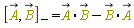
Commutators and Anticommutators of vectorial quantum operators `#mover(mi("A",mathcolor = "olive"),mo("&rarr;"))`, `#mover(mi("B",mathcolor = "olive"),mo("&rarr;"))`, are now implemented and expressed using the dot (scalar) product, as in Physics:-Commutator(`#mover(mi("A",mathcolor = "olive"),mo("&rarr;"))`, `#mover(mi("B",mathcolor = "olive"),mo("&rarr;"))`) = `#mover(mi("A",mathcolor = "olive"),mo("&rarr;"))`.`#mover(mi("B",mathcolor = "olive"),mo("&rarr;"))`-`#mover(mi("B",mathcolor = "olive"),mo("&rarr;"))`.`#mover(mi("A",mathcolor = "olive"),mo("&rarr;"))`
• 

If two noncommutative operators a and S  satisfy "[a^(&dagger;),S][-]=0" , then the commutator  "[a,S^(&dagger;)][-]" is automatically taken equal to 0; if in addition S is Hermitian, then  "[a,S][-]"is also automatically taken equal to zero.

Examples


Expand and Combine


In the context of Physics, the expansion and recombination of algebraic expressions requires additional care: products may involve non-commutative operators and then some of the standard expansion and combination rules do not apply, or apply differently. Similarly, the expansion of vectorial operators also follows special rules. During 2013, many of these algebraic operations were reviewed and related special formulas (such as Glauber's and Haussdorf's) were implemented.

Examples


New Enhanced Modes in Physics Setup


Four enhanced modes were added to the Physics setup. With these modes, you can:

1. 

Indicate the real objects of a computation.

2. 

Automatically combine powers of the same base.

3. 

Set Maple to take z and its conjugate, "z," as independent variables and in equal footing; this is Wirtinger calculus.

4. 

Redefine the sum command in order to perform multi-index summation.

These options combined provide flexibility, subsequently making the Physics environment more expressive.

Real Objects


Combining Powers of the Same Base


Complex variables: z and conjugate(z) in equal footing


Redefine Sum for Multi-Index Summation


Dagger


Physics:-Dagger now has the same shortcut notation of Hermitian transpose , which acts on Vectors, vector products, equations, and automatically maps over the arguments of derivatives when the differentiation variables are real.

Examples


Vectors Package


A number of changes were performed in the Vectors subpackage to make the computations more natural and versatile:

• 

You can now use geometrical coordinates indexed, as in r[j], to represent mathematical objects unrelated to the coordinates themselves (in this case the spherical coordinate r).  This is a more appropriate mimicry of the way we compute with paper and pencil.

• 

Integrate the Vectors package commands with assuming and accept a tensor with 1 index (of type Library:-PhysicsType:-Tensor, defined using Define) as a possible abstract representation of the kth component of a vector.

• 

When V is a vector of the Physics:-Vectors package, make its absolute value abs(V), compute automatically using Physics:-Vectors:-Norm

• 

For an arbitrary vector  `#mover(mi("A"),mo("&rarr;"))`, make its Norm LinearAlgebra[Norm](`#mover(mi("A"),mo("&rarr;"))`) = "A*(A)," and introduce a new option conjugate to Norm, to specify whether to use `#mover(mi("A"),mo("&rarr;"))`.conjugate(`#mover(mi("A"),mo("&rarr;"))`) or `#mover(mi("A"),mo("&rarr;"))`.`#mover(mi("A"),mo("&rarr;"))` when computing LinearAlgebra[Norm](`#mover(mi("A"),mo("&rarr;"))`).

• 

When `#mover(mi("A",mathcolor = "olive"),mo("&rarr;"))` is a quantum operator, Norm returns using Dagger instead of conjugate.

• 

Commutators and Anticommutators of vectorial quantum operators `#mover(mi("A",mathcolor = "olive"),mo("&rarr;"))`, `#mover(mi("B",mathcolor = "olive"),mo("&rarr;"))`, are now implemented and expressed using the dot (scalar) product, as in "[A,B][-]=A*B-B*A . "

• 

New PhysicsVectors type in the Library of types Library:-PhysicsTypes, in order to programmatically identify vectors of the Physics:-Vectors package.


Two examples illustrating the use of the new capabilities in the context of a more general problem are found in the MaplePrimes posts Quantum Mechanics using Computer Algebra and Quantum Mechanics (II).

Examples


Library


Seventeen new commands, useful for programming and interactive computation, were added to the Physics:-Library package. These are:

• 

Add unifies the standard add and sum commands using a more modern handling of arguments, free of premature evaluation problems, and brings new multi-index functionality.

• 

ApplyCommandUsingImplicitAssumptions applies any command to expressions containing sums, integrals or products such that the command is applied to the summand (integrand or 1st argument of the product) taking into account the assumptions implicit in the summation (integration or product) range.

• 

CombinePowersOfSameBase combines powers of the same base in products correctly handling the case of noncommutative products and powers, using Glauber's formula.

• 

FromTensorFunctionalForm is a generalization of the former FromGeneralRelativityTensorFunctionalForm command, that also handles user defined tensor functions.

• 

GetFAndDifferentiationVariables receives a derivative and returns a sequence with derivand and all the differentiation variables.

• 

GetReplacementIndices receives a list of indices of different kinds (spacetime, space, spinor, etc) and any other arguments and returns a list with new indices of the same kinds - useful for replacements - not present in the rest of the arguments.

• 

GetSymbolsWithSameType receives an expression x, of type commutative, anticommutative or noncommutative, and any other arguments, and returns symbols of the same type as x, and not present in the rest of arguments.

• 

GetTensorDependency gets the dependency of a given tensor; this dependency typically depends of the spacetime metric or on the way you defined the tensor using Define.

• 

GetTensorFunctionalForm is a generalization of the former GetGeneralRelativityTensorFunctionalForm command, that also handles user defined tensor functions.

• 

IsLiteralSubscript returns true or false according to whether a symbol s is of the form x__y, that is, it has the substring __ after the first or next characters and before the last one.

• 

IsRealObject returns true or false according to whether a mathematical expression, function or variable passed is known to be real, either because it was assumed to be real, or because it was set to be real using Setup and its realobjects keyword.

• 

RealObjects sets and unsets mathematical variables and functions as real, and answers queries about them.

• 

SortProducts sorts the operands of noncommutative products into any particular desired ordering while taking into account commutator and anticommutator algebra rules, such that the returned product is mathematically equivalent to the one received.

• 

SubstituteTensor substitutes equations into an expression, taking care of the free and repeated indices such that: 1) the substitution equations are interpreted as mappings having the free indices as parameters, and 2) repeated indices in the substitution equations do not clash with existing repeated indices in the target expression.

• 

ToContravariant and ToCovariant rewrite a given expression multiplying by the spacetime metric so that all of its free indices become respectively contravariant or covariant.

• 

ToTensorFunctionalForm reverses the operation performed by the new FromTensorFunctionalForm described above.

Examples


Miscellaneous

 
• 

Implement formulas for abstract k, n both nonnegint entering "`a+`^k*| A[n] >" and "a(-)^k*| A[n] >", where `a+` and "a-" are Creation and Annihilation operators, respectively, acting on the 1st quantum number of the space of quantum states labeled A.

• 

Implement new PDEtools:-dchange rules for changing variables in Bras Kets and Brackets of the Physics package

• 

Library:-Degree can now compute the degree for noncommutative products Enhance PDEtools:-Library:-Degree and PDEtools:-Coefficients, to work with Physics:-`.` the same way it does with Physics:-`*`

• 

Changes in design:

a. 

When the spacetime is Euclidean, there is no difference in value between the covariant and contravariant components of a tensor. Therefore, represent both with covariant indices making simplification and all manipulations simpler. This change affects the display of indices on the screen as well as the output of SumOverRepeatedIndices.

b. 

The dot product A . B of quantum operators A and B now returns as a (noncommutative) product  A * B when neither A nor B involve Bras or Kets.

c. 

When A is a quantum operator (generic, Hermitian or unitary), the literal subscript object A__x is now considered an operator of the same kind.

d. 

Normal normalizes powers of the same base (including exponentials) by combining them. For example, A^n*A^m "->A^(n+m)."

e. 

Normal normalizes noncommutative products by sorting objects that commute between themselves putting those that involve Dagger and conjugate to the left, more aligned with normal ordering in quantum field theories.

f. 

FeynmanDiagrams does not return any crossed propagators unless explicitly requested using the new option includecrossedpropagators. The former option, normalproducts, was renamed as externallegs.

Examples


See Also


The Physics project, Physics, what is new in Physics in Maple 17, what is new in Physics in Maple 16


Physics2013.pdf    Physics2013.mw

Edgardo S. Cheb-Terrab
Physics, Maplesoft

Hi

It's been 3+ months since we launched this new, experimental, Maple Physics: Research & Development webpage, containing fixes and new developments around the clock made available to everybody. Today we are extending this experience to Differential Equations and Mathematical functions, launching the Maple Differential Equations and Mathematical Functions: Research & Development Maplesoft webpage. Hey!

With these pages we intend to move the focus of developments directly into the topics people are actually working on. The experience so far has been really good, putting our development at high RPM, an exciting roller-coast of exchange and activity.

As with the Research version of Physics, when suggestions about DEs or Mathematical Functions are implemented or issues are fixed, typically within a couple of days when that is possible, the changes will be made available to everybody directly in this new Maplesoft webpage. One word of clarification: for now, these updates will not include numerical ODE or numerical PDE solutions nor their numerical plotting. Sorry guys. One step at a time :)

This first update today concerns Differential Equations: dsolve and pdsolve can now handle linear systems of equations also when entered in Vector notation (Matrices and Vectors), related to a post in Mapleprimes from October/29. Attached is a demo illustrating the idea.

Everybody is welcome to bring suggestions and post issues. You can do that directly in Mapleprimes or writing to physics@maplesoft.com. While Differential Equations and Mathematical Functions are two areas where the Maple system is currently more mature than in Physics, these two areas cover so many subjects, including that there are the Research and the Education perspectives, that the number of possible topics is immense. 

DEsAndMathematicalFu.pdf   DEsAndMathematicalFu.mw

Edgardo S. Cheb-Terrab
Physics, DEs and Mathematical Functions, Maplesoft

First 14 15 16 17 18 Page 16 of 18



