ecterrab

14837 Reputation

24 Badges

21 years, 88 days

MaplePrimes Activity


These are Posts that have been published by ecterrab


Minimize the number of tensor components according to its symmetries
(and relabel, redefine or count the number of independent tensor components)


The nice development described below is work in collaboration with Pascal Szriftgiser from Laboratoire PhLAM, Université Lille 1, France, used in the Mapleprimes post Magnetic traps in cold-atom physics


A new keyword in Define  and Setup : minimizetensorcomponents, allows for automatically minimizing the number of tensor components taking into account the tensor symmetries. For example, if a tensor with two indices in a 4D spacetime is defined as antisymmetric using Define with this new keyword, the number of different tensor components will be exactly 6, and the elements of the diagonal are automatically set equal to 0. After setting this keyword to true with Setup , all subsequent definitions of tensors automatically minimize the number of components while using this keyword with Define  makes this minimization only happen with the tensors being defined in the call to Define .


Related to this new functionality, 4 new Library routines were added: MinimizeTensorComponents, NumberOfIndependentTensorComponents, RelabelTensorComponents and RedefineTensorComponents


Example:

> 

restart; with(Physics)


Define an antisymmetric tensor with two indices

> 

Define(F[mu, nu], antisymmetric)

`Defined objects with tensor properties`


{Physics:-Dgamma[mu], F[mu, nu], Physics:-Psigma[mu], Physics:-d_[mu], Physics:-g_[mu, nu], Physics:-KroneckerDelta[mu, nu], Physics:-LeviCivita[alpha, beta, mu, nu]}

(1.1)

Although the system knows that F[mu, nu] is antisymmetric, you need to use Simplify to apply the (anti)symmetry

> 

F[mu, nu]+F[nu, mu]

F[mu, nu]+F[nu, mu]

(1.2)


> 

Simplify(F[mu, nu]+F[nu, mu])

0

(1.3)

so by default the components of F[mu, nu] do not automatically reflect the (anti)symmetry; likewise

> 

F[1, 2]+F[2, 1]

F[1, 2]+F[2, 1]

(1.4)
> 

Simplify(F[1, 2]+F[2, 1])

0

(1.5)

and computing the array form of F[mu, nu]we do not see the elements of the diagonal equal to zero nor the lower-left triangle equal to the upper-right triangle but for a different sign:

> 

TensorArray(F[mu, nu])

Matrix(%id = 18446744078270093062)

(1.6)


On the other hand, this new functionality, here called minimizetensorcomponents, makes the symmetries of the tensor be explicitly reflected in its components.


There are three ways to use it. First, one can minimize the number of tensor components of a tensor previously defined. For example


> 

Library:-MinimizeTensorComponents(F)

Matrix(%id = 18446744078270064630)

(1.7)

After this, both (1.2) and (1.3) are automatically equal to 0 without having to use Simplify

> 

F[mu, nu]+F[nu, mu]

0

(1.8)
> 

0

0

(1.9)

And the output of TensorArray  in (1.6) becomes equal to (1.7).


NOTE: in addition, after using minimizetensorcomponents in the definition of a tensor, say F, all the keywords implemented for Physics tensors are available for F:


> 

F[]

F[mu, nu] = Matrix(%id = 18446744078247910206)

(1.10)
> 

F[trace]

0

(1.11)
> 

F[nonzero]

F[mu, nu] = {(1, 2) = F[1, 2], (1, 3) = F[1, 3], (1, 4) = F[1, 4], (2, 1) = -F[1, 2], (2, 3) = F[2, 3], (2, 4) = F[2, 4], (3, 1) = -F[1, 3], (3, 2) = -F[2, 3], (3, 4) = F[3, 4], (4, 1) = -F[1, 4], (4, 2) = -F[2, 4], (4, 3) = -F[3, 4]}

(1.12)
> 

"F[~1,mu,matrix]"

F[`~1`, mu] = Vector[row](%id = 18446744078247885990)

(1.13)

Alternatively, one can define a tensor, specifying that the symmetries should be taken into account to minimize the number of its components passing the keyword minimizetensorcomponents to Define .


Example:


Define a tensor with the symmetries of the Riemann  tensor, that is, a tensor of 4 indices that is symmetric with respect to interchanging the positions of the 1st and 2nd pair of indices and antisymmetric with respect to interchanging the position of its 1st and 2nd indices, or 3rd and 4th indices, and define it minimizing the number of tensor components


> 

Define(R[alpha, beta, mu, nu], symmetric = {[[1, 2], [3, 4]]}, antisymmetric = {[1, 2], [3, 4]}, minimizetensorcomponents)

`Defined objects with tensor properties`


{Physics:-Dgamma[mu], F[mu, nu], Physics:-Psigma[mu], R[mu, nu, alpha, beta], Physics:-d_[mu], Physics:-g_[mu, nu], Physics:-KroneckerDelta[mu, nu], Physics:-LeviCivita[alpha, beta, mu, nu]}

(1.14)

We now have

> 

R[1, 2, 3, 4]+R[2, 1, 3, 4]

0

(1.15)
> 

R[alpha, beta, mu, nu]-R[mu, nu, alpha, beta]

0

(1.16)
• 

One can always retrieve the symmetry properties in the abstract notation used by the Define command using the new Library:-GetTensorSymmetryProperties, its output is ordered, first the symmetric then the antisymmetric properties


> 

Library:-GetTensorSymmetryProperties(R)

{[[1, 2], [3, 4]]}, {[1, 2], [3, 4]}

(1.17)
• 

After making the symmetries explicit (and also before that), it is frequently useful to know the number of independent components of a given tensor. For this purpose you can use the new Library:-NumberOfIndependentTensorComponents


> 

Library:-NumberOfIndependentTensorComponents(R)

21

(1.18)

and besides taking into account the symmetries, in the case of the Riemann  tensor, after taking into account the first Bianchi identity this number of components is further reduced to 20.


A third way of using the new minimizetensorcomponents functionality is using Setup , so that, automatically, every subsequent definition of tensors with symmetries is performed minimizing the number of its components using the indicated symmetries


Example:

> 

Setup(minimizetensorcomponents = true)

[minimizetensorcomponents = true]

(1.19)

So from hereafter you can define tensors taking into account their symmetries explicitly and without having to include the keyword minimizetensorcomponents at each definition


> 

Define(C[alpha, beta], antisymmetric)

`Defined objects with tensor properties`


{C[mu, nu], Physics:-Dgamma[mu], F[mu, nu], Physics:-Psigma[mu], R[mu, nu, alpha, beta], Physics:-d_[mu], Physics:-g_[mu, nu], Physics:-KroneckerDelta[mu, nu], Physics:-LeviCivita[alpha, beta, mu, nu]}

(1.20)


> 

C[]

C[mu, nu] = Matrix(%id = 18446744078408747598)

(1.21)
• 

Two new related functionalities are provided via Library:-RelabelTensorComponents and Library:-RedefineTensorComponent, the first one to have the number of tensor components directly reflected in the names of the components, the second one to redefine only one of these components

> 

Library:-RelabelTensorComponents(C)

Matrix(%id = 18446744078408729774)

(1.22)


Suppose now we want to make one of these components equal to 1, say C__2

> 

Library:-RedefineTensorComponent(C[1, 2] = 1)

C[mu, nu] = Matrix(%id = 18446744078270104390)

(1.23)

This nice development is work in collaboration with Pascal Szriftgiser from Laboratoire PhLAM, UMR CNRS 8523, Université Lille 1, F-59655, France.

> 

``


Download MinimizeTensorComponents.mw


Edgardo S. Cheb-Terrab
Physics, Differential Equations and Mathematical Functions, Maplesoft

It passed through my mind it would be interesting to collect the links to the most relevant Mapleprimes posts about Quantum Mechanics using the Physics package of the last couple of years, to have them all accessible from one place. These posts give an idea of what kind of computation is already doable in quantum mechanics, how close is the worksheet input to what we write with paper and pencil, and how close is the typesetting of the output to what we see in textbooks.

At the end of each page linked below, you will see another link to download the corresponding worksheet, that you can open using Maple (say the current version or the version 1 or 2 years ago).

This other set of three consecutive posts develops one problem split into three parts:

This other link is interesting as a quick and compact entry point to the use of the Physics package:

There is an equivalent set of Mapleprimes posts illustrating the Physics package tackling problems in General Relativity, collecting them is for one other time.

Edgardo S. Cheb-Terrab
Physics, Differential Equations and Mathematical Functions, Maplesoft

December 2017: This is, perhaps, one of the most complicated computations done in this area using the Physics package. To the best of my knowledge never before performed on a computer algebra worksheet. It is exciting to present a computation like this one. At the end the corresponding worksheet is linked so that it can be downloaded and the sections be opened, the computation be reproduced. There is also a link to a pdf with everything open.  Special thanks to Pascal Szriftgiser for bringing this problem. To reproduce the computations below, please update the Physics library with the one distributed from the Maplesoft R&D Physics webpage.

June 17, 2020: updated taking advantage of new features of Maple 2020.1 and Physics Updates v.705. Submitted to arxiv.org. 

January 25, 2021: updated in the arXiv and submitted for publication in Computer Physics Communications. 


Quantum Runge-Lenz Vector and the Hydrogen Atom,

the hidden SO(4) symmetry using Computer Algebra


Pascal Szriftgiser1 and Edgardo S. Cheb-Terrab2 

(1) University of Lille, CNRS, UMR 8523 - PhLAM - Physique des Lasers, Atomes et Molécules, F-59000 Lille, France

(2) Maplesoft

NULL


Abstract


Pauli first noticed the hidden SO(4) symmetry for the Hydrogen atom in the early stages of quantum mechanics [1]. Departing from that symmetry, one can recover the spectrum of a spinless hydrogen atom and the degeneracy of its states without explicitly solving Schrödinger's equation [2]. In this paper, we derive that SO(4) symmetry and spectrum using a computer algebra system (CAS). While this problem is well known [3, 4], its solution involves several steps of manipulating expressions with tensorial quantum operators, simplifying them by taking into account a combination of commutator rules and Einstein's sum rule for repeated indices. Therefore, it is an excellent model to test the current status of CAS concerning this kind of quantum-and-tensor-algebra computations. Generally speaking, when capable, CAS can significantly help with manipulations that, like non-commutative tensor calculus subject to algebra rules, are tedious, time-consuming and error-prone. The presentation also shows a pattern of computer algebra operations that can be useful for systematically tackling more complicated symbolic problems of this kind.


Introduction


The primary purpose of this work is to derive, step-by-step, the SO(4) symmetry of the Hydrogen atom and its spectrum using a computer algebra system (CAS). To the best of our knowledge, such a derivation using symbolic computation has not been shown before. Part of the goal was also to see whether this computation can be performed entering only the main definition formulas, followed by only simplification commands, and without using previous knowledge of the result. The intricacy of this problem is in the symbolic manipulation and simplification of expressions involving noncommutative quantum tensor operators. The simplifications need to take into account commutator rules, symmetries under permutation of indices of tensorial subexpressions, and use Einstein's sum rule for repeated indices.

We performed the derivation using the Maple 2020 system with the Maplesoft Physics Updates v.705. Generally speaking, the default computational domain of CAS doesn't include tensors, noncommutative operators nor related simplifications. On the other hand, the Maple system is distributed with a Physics package that extends that default domain to include those objects and related operations. Physics includes a Simplify command that takes into account custom algebra rules and the sum rule for repeated indices, and uses tensor-simplification algorithms [5] extended to the noncommutative domain.


A note about notation: when working with a CAS, besides the expectation of achieving a correct result for a complicated symbolic calculation, readability is also an issue. It is desired that one be able to enter the definition formulas and computational steps to be performed (the input, preceded by a prompt >, displayed in black) in a way that resembles as closely as possible their paper and pencil representation, and that the results (the output, computed by Maple, displayed in blue) use textbook mathematical-physics notation. The Physics package implements such dedicated typesetting. In what follows, within text and in the output, noncommutative objects are displayed using a different color, e.g. H, vectors and tensor indices are displayed the standard way, as in `#mover(mi("L",mathcolor = "olive"),mo("→"))`, and L[q], and commutators are displayed with a minus subscript, e.g. "[H,L[q]][-]". Although the Maple system allows for providing dedicated typesetting also for the input, we preferred to keep visible the Maple input syntax, allowing for comparison with paper and pencil notation. We collected the names of the commands used and a one line description for them in an Appendix at the end. Maple also implements the concept of inert representations of computations, which are activated only when desired. We use this feature in several places. Inert computations are entered by preceding the command with % and are displayed in grey. Finally, as is usual in CAS, every output has an equation label, which we use throughout the presentation to refer to previous intermediate results.


In Sec.1, we recall the standard formulation of the problem and present the computational goal, which is the derivation of the formulas representing the SO(4) symmetry and related spectrum.


In Sec.2, we set tensorial non-commutative operators representing position and linear and angular momentum, respectively X[a], p[a] and L[a], their commutation rules used as departure point, and the form of the quantum Hamiltonian H. We also derive a few related identities used in the sections that follow.


In Sec.3, we derive the conservation of both angular momentum and the Runge-Lenz quantum operator, respectively "[H,L[q]][-]=0" and "[H,Z[k]][-]=0". Taking advantage of the differentialoperators functionality in the Physics package, we perform the derivation exploring two equivalent approaches; first using only a symbolic tensor representation p[j] of the momentum operator, then using an explicit differential operator representation for it in configuration space, p[j] = -i*`ℏ`*`∂`[j].  With the first approach, expressions are simplified only using the departing commutation rules and Einstein's sum rule for repeated indices. Using the second approach, the problem is additionally transformed into one where the differentiation operators are applied explicitly to a test function G(X). Presenting both approaches is of potential interest as it offers two partly independent methods for performing the same computation, which is helpful to provide confidence on in the results when unknown, a relevant issue when using computer algebra.


In Sec. 4, we derive %Commutator(L[m], Z[n]) = I*`ℏ`*`ε`[m, n, u]*Z[u] and show that the classical relation between angular momentum and the Runge-Lenz vectors,  "L *"`#mover(mi("Z"),mo("→"))` = 0, due to the orbital momentum being perpendicular to the elliptic plane of motion while the Runge-Lenz vector lies in that plane, still holds in quantum mechanics, where the components of these quantum vector operators do not commute but "L *"`#mover(mi("Z",mathcolor = "olive"),mo("→"))` = "(Z) *"`#mover(mi("L",mathcolor = "olive"),mo("→"))` = 0.


In Sec. 5, we derive "[Z[a],Z[b]][-]=-(2 i `ℏ` `ε`[a,b,c] (H L[c]))/`m__e`" using the two alternative approaches described for Sec.3.

In Sec. 6, we derive the well-known formula for the square of the Runge-Lenz vector, Z[k]^2 = 2*H*(`ℏ`^2+L[a]^2)/m__e+kappa^2.


Finally, in Sec. 7, we use the SO(4) algebra derived in the previous sections to obtain the spectrum of the Hydrogen atom. Following the literature, this approach is limited to the bound states for which the energy is negative.


Some concluding remarks are presented at the end, and input syntax details are summarized in an Appendix.


1. The hidden SO(4) symmetry of the Hydrogen atom


Let's consider the Hydrogen atom and its Hamiltonian

H = LinearAlgebra[Norm](`#mover(mi("p"),mo("→"))`)^2/(2*m__e)-kappa/r,


where `#mover(mi("p"),mo("→"))`is the electron momentum, m__e its mass, κ a real positive constant, r = `≡`(LinearAlgebra[Norm](`#mover(mi("r"),mo("→"))`), sqrt(X[a]^2)) the distance of the electron from the proton located at the origin, and X[a] is its tensorial representation with components ["x, y,z]". We assume that the proton's mass is infinite. The electron and nucleus spin are not taken into account. Classically, from the potential -kappa/r, one can derive a central force `#mover(mi("F"),mo("→"))` = -kappa*`#mover(mi("r"),mo("∧"))`/r^2 that drives the electron's motion. Introducing the angular momentum


`#mover(mi("L"),mo("→"))` = `&x`(`#mover(mi("r"),mo("→"))`, `#mover(mi("p"),mo("→"))`),


one can further define the Runge-Lenz vector `#mover(mi("Z"),mo("→"))`


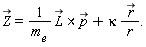
"Z=1/(`m__e`) (L)*(p)+kappa ( r)/r."


It is well known that `#mover(mi("Z"),mo("→"))` is a constant of the motion, i.e. diff(`#mover(mi("Z"),mo("→"))`(t), t) = 0. Switching to Quantum Mechanics, this condition reads


%Commutator(H, Z_) = 0.


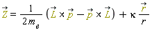
where, for hermiticity purpose, the expression of `#mover(mi("Z",mathcolor = "olive"),mo("→"))` must be symmetrized


`#mover(mi("Z",mathcolor = "olive"),mo("→"))` = (`&x`(`#mover(mi("L",mathcolor = "olive"),mo("→"))`, `#mover(mi("p",mathcolor = "olive"),mo("→"))`)-`&x`(`#mover(mi("p",mathcolor = "olive"),mo("→"))`, `#mover(mi("L",mathcolor = "olive"),mo("→"))`))/(2*m__e)+kappa*`#mover(mi("r",mathcolor = "olive"),mo("→"))`/r.


In what follows, departing from the Hamiltonian H, the basic commutation rules between position`#mover(mi("r",mathcolor = "olive"),mo("→"))`, momentum `#mover(mi("p",mathcolor = "olive"),mo("→"))` and angular momentum `#mover(mi("L",mathcolor = "olive"),mo("→"))` in tensor notation, we derive the following commutation rules between the quantum Hamiltonian, angular momentum and Runge-Lenz vector `#mover(mi("Z",mathcolor = "olive"),mo("→"))`


"[H,L[n]][-]"

=

0

"[H,Z[n]][-]"

=

0

" [L[m],Z[n]][-]"

=

I*`ℏ`*`ε`[m, n, o]*Z[o]

" [Z[m],Z[n]][-]"

=

-(2*(I*`ℏ`/m__e))*H*`ε`[m, n, o]*L[o]


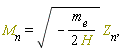
Since H commutes with both `#mover(mi("L",mathcolor = "olive"),mo("→"))`NULL and `#mover(mi("Z",mathcolor = "olive"),mo("→"))`, defining


"`M__n`=sqrt(-(`m__e`)/(2 H)) `Z__n`,"

these commutation rules can be rewritten as


"[L[m],L[n]][-]"

=

I*`ℏ`*`ε`[m, n, o]*L[o]

" [L[m],M[n]][-]"

=

I*`ℏ`*`ε`[m, n, o]*M[o]

"[M[m],M[n]][-]"

=

I*`ℏ`*`ε`[m, n, o]*L[o]


This set constitutes the Lie algebra of the SO(4) group.


2. Setting the problem, commutation rules and useful identities


3. Commutation rules between the Hamiltonian and each of the angular momentum and Runge-Lenz tensors


4. Commutation rules between the angular momentum L[q]and the Runge-Lenz Z[k]tensors


5.  Commutation rules between the components of the Runge-Lenz tensor


6. The square of the norm of the Runge-Lenz vector


7. The atomic hydrogen spectrum


Conclusions


In this presentation, we derived, step-by-step, the SO(4) symmetry of the Hydrogen atom and its spectrum using the symbolic computer algebra Maple system. The derivation was performed without departing from the results, entering only the main definition formulas in eqs. (1), (2) and (5), followed by using a few simplification commands - mainly Simplify, SortProducts and SubstituteTensor - and a handful of Maple basic commands, subs, lhs, rhs and isolate. The computational path that was used to get the results of sections 2 to 7 is not unique. Instead of searching for the shortest path, we prioritized clarity and illustration of the techniques that can be used to crack problems like this one.

This problem is mainly about simplifying expressions using two different techniques. First, expressions with noncommutative operands in products need reduction with respect to the commutator algebra rules that have been set. Second, products of tensorial operators require simplification using the sum rule for repeated indices and the symmetries of tensorial subexpressions. Those techniques, which are part of the Maple Physics simplifier, together with the SortProducts and SubstituteTensor commands for sorting the operands in products to apply tensorial identities, sufficed. The derivations were performed in a reasonably small number of steps.

Two different computational strategies - with and without differential operators - were used in sections 3 and 5, showing an approach for verifying results, a relevant issue in general when performing complicated algebraic manipulations. The Maple Physics ability to handle differential operators as noncommutative operands in products (as frequently done in paper and pencil computations) facilitates readability and ease in entering the computations. The complexity of those operations is then handled by one Physics:-Library command, ApplyProductsOfDifferentialOperators (see eqs. (47) and (83)).

Besides the Maple Physics ability to handle noncommutative tensor operators and simplify such operators using commutator algebra rules, it is interesting to note: a) the ability of the system to factorize expressions involving products of noncommutative operands (see eqs. (90) and (108)) and b) the extension of the algorithms for simplifying tensorial expressions [5] to the noncommutativity domain, used throughout this presentation.

It is also worth mentioning how equation labels can reduce the whole computation to entering the main definitions, followed by applying a few commands to equation labels. That approach helps to reduce the chance of typographical errors to a very strict minimum. Likewise, the fact that commands and equations distribute over each other allows cumbersome manipulations to be performed in simple ways, as done, for instance, in eqs. (8), (9) and (13).

Finally, it was significantly helpful for us to have the typesetting of results using standard mathematical physics notation, as shown in the presentation above.


Appendix


In this presentation, the input lines are preceded by a prompt > and the commands used are of three kinds: some basic Maple manipulation commands, the main Physics package commands to set things and simplify expressions, and two commands of the Physics:-Library to perform specialized, convenient, operations in expressions.


The basic Maple commands used


• 

interface is used once at the beginning to set the letter used to represent the imaginary unit (default is I but we used i).

• 

isolate is used in several places to isolate a variable in an expression, for example isolating x in a*x+b = 0 results in x = -b/a

• 

lhs and rhs respectively get the left-hand side Aand right-hand side Bof an equation A = B

• 

subs substitutes the left-hand side of an equation by the righ-hand side in a given target, for example subs(A = B, A+C) results in B+C

• 

@ is used to compose commands. So(`@`(A, B))(x) is the same as A(B(x)). This command is useful to express an abstract combo of manipulations, for example as in (108) ≡ lhs = `@`(Factor, rhs).


The Physics commands used


• 

Setup is used to set algebra rules as well as the dimension of space, type of metric, and conventions as the kind of letter used to represent indices.

• 

Commutator computes the commutator between two objects using the algebra rules set using Setup. If no rules are known to the system, it outputs a representation for the commutator that the system understands.

• 

CompactDisplay is used to avoid redundant display of the functionality of a function.

• 

d_[n] represents the `∂`[n] tensorial differential operator.

• 

Define is used to define tensors, with or without specifying its components.

• 

Dagger  computes the Hermitian transpose of an expression.

• 

Normal, Expand, Factor respectively normalizes, expands and factorizes expressions that involve products of noncommutative operands.

• 

Simplify performs simplification of tensorial expressions involving products of noncommutative factors taking into account Einstein's sum rule for repeated indices, symmetries of the indices of tensorial subexpressions and custom commutator algebra rules.

• 

SortProducts uses the commutation rules set using Setup to sort the non-commutative operands of a product in an indicated ordering.


The Physics:-Library commands used


• 

Library:-ApplyProductsOfDifferentialOperators applies the differential operators found in a product to the product operands that appear to its right. For example, applying this command to  p*V(X)*m__e results in m__e*p(V(X))

• 

Library:-EqualizeRepeatedIndices equalizes the repeated indices in the terms of a sum, so for instance applying this command to L[a]^2+L[b]^2 results in 2*L[a]^2


References


[1] W. Pauli, "On the hydrogen spectrum from the standpoint of the new quantum mechanics,” Z. Phys. 36, 336–363 (1926)

[2] S. Weinberg, "Lectures on Quantum Mechanics, second edition, Cambridge University Press," 2015.

[3] Veronika Gáliková, Samuel Kováčik, and Peter Prešnajder, "Laplace-Runge-Lenz vector in quantum mechanics in noncommutative space", J. Math. Phys. 54, 122106 (2013)

[4] Castro, P.G., Kullock, R. "Physics of the so__q(4) hydrogen atom". Theor. Math. Phys. 185, 1678–1684 (2015).

[5] L. R. U. Manssur, R. Portugal, and B. F. Svaiter, "Group-Theoretic Approach for Symbolic Tensor Manipulation," International Journal of Modern Physics C, Vol. 13, No. 07, pp. 859-879 (2002).


Download Hidden_SO4_symmetry_of_the_hydrogen_atom.mw

Download Hidden_SO4_symmetry_submitted_to_CPC.pdf (all sections open)


Edgardo S. Cheb-Terrab
Physics, Differential Equations and Mathematical Functions, Maplesoft

The computation of traces of products of Dirac matrices was implemented years ago - see Physics,Trace .


The simplification of products of Dirac matrices, however, was not. Now it is, and illustrating this new feature is the matter of this post. To reproduce the results below please update the Physics library with the one distributed at the Maplesoft R&D Physics webpage.

> 

with(Physics)


First of all, when loading Physics, a frequent question is about the signature, the default is (- - - +)

> 

Setup(signature)

[signature = `- - - +`]

(1)

This is important because the convention for the Algebra of Dirac Matrices depends on the signature. With the signatures (- - - +) as well as (+ - - -), the sign of the timelike component is 1

> 

Library:-SignOfTimelikeComponent()

1

(2)

With the signatures (+ + + -) as well as (- + + +), the sign of the timelike component is of course -1

> 

Library:-SignOfTimelikeComponent(`+ + + -`)

-1

(3)

The simplification of products of Dirac Matrices, illustrated below with the default signature, works fine with any of these signatures, and works without having to set a representation for the Dirac matrices -- all the results are representation-independent.


The examples below, however, also illustrate a new feature of Physics, for now implemented as a Library:-PerformMatrixOperations command (there is a related, also new, command, Library:-RewriteInMatrixForm, to just present the underlying matrix operations, without performing them). To illustrate this other new functionality , set a representation for the Dirac matrices, say the standard one


> 

Setup(Dgamma = standard, math = true)

`* Partial match of  'Physics:-Dgamma' against keyword 'Dgammarepresentation'`


`* Partial match of  'math' against keyword 'mathematicalnotation'`


`Setting lowercaselatin letters to represent spinor indices `


`Defined Dirac gamma matrices (Dgamma) in standard representation`, gamma[1], gamma[2], gamma[3], gamma[4]


__________________________________________________


[Dgammarepresentation = standard, mathematicalnotation = true]

(4)

The four Dirac matrices are

> 

TensorArray(Dgamma[`~mu`])

Array(%id = 18446744078360533342)

(5)

The definition of the Dirac matrices is implemented in Maple following the conventions of Landau books ([1] Quantum Electrodynamics, V4), and  does not depend on the signature, ie the form of these matrices is

> 

"Library:-RewriteInMatrixForm(?)"

Array(%id = 18446744078360529726)

(6)

With the default signature, the space part components of  gamma[mu] change sign when compared with corresponding ones from gamma[`~mu`] while the timelike component remains unchanged

> 

TensorArray(Dgamma[mu])

Array(%id = 18446744078565663678)

(7)
> 

"Library:-RewriteInMatrixForm(?)"

Array(%id = 18446744078677131982)

(8)

For the default signature, the algebra of the Dirac Matrices, loaded by default when Physics is loaded, is (see page 80 of [1])

> 

(%AntiCommutator = AntiCommutator)(Dgamma[`~mu`], Dgamma[`~nu`])

%AntiCommutator(Physics:-Dgamma[`~mu`], Physics:-Dgamma[`~nu`]) = 2*Physics:-g_[`~mu`, `~nu`]

(9)

When the sign of the timelike component of the signature is -1, we have a -1 factor on the right-hand side of (9).


Note as well that in (9) the right-hand side has no matrix elements. This is standard in particle physics where the computations are performed algebraically, without performing the matrix operations. For the purpose of actually performing the underlying matrix operations, however, one may want to rewrite this algebra including a 4x4 identity matrix. For that purpose, see Algebra of Dirac Matrices with an identity matrix on the right-hand side. For the purpose of this illustration, below we proceed with the algebra as shown in (9), interpreting right-hand sides as if they involve an identity matrix.


Verify the algebra rule by performing all the involved matrix operations

> 

expand(%AntiCommutator(Physics[Dgamma][`~mu`], Physics[Dgamma][`~nu`]) = 2*Physics[g_][`~mu`, `~nu`])

Physics:-`*`(Physics:-Dgamma[`~mu`], Physics:-Dgamma[`~nu`])+Physics:-`*`(Physics:-Dgamma[`~nu`], Physics:-Dgamma[`~mu`]) = 2*Physics:-g_[`~mu`, `~nu`]

(10)

Note that, regarding the spacetime indices, this is a 4x4 matrix, whose elements are in turn 4x4 matrices. Compute first the external 4x4 matrix related to mu and nu

> 

TensorArray(Physics[`*`](Physics[Dgamma][`~mu`], Physics[Dgamma][`~nu`])+Physics[`*`](Physics[Dgamma][`~nu`], Physics[Dgamma][`~mu`]) = 2*Physics[g_][`~mu`, `~nu`])

Matrix(%id = 18446744078587020822)

(11)

Perform now all the matrix operations involved in each of the elements of this 4x4 matrix

> 

"Library:-PerformMatrixOperations(?)"

Matrix(%id = 18446744078743243942)

(12)

By eye everything checks OK.NULL


Consider now the following five products of Dirac matrices

> 

e0 := Dgamma[mu]^2

Physics:-`*`(Physics:-Dgamma[mu], Physics:-Dgamma[`~mu`])

(13)
> 

e1 := Dgamma[mu]*Dgamma[`~nu`]*Dgamma[mu]

Physics:-`*`(Physics:-Dgamma[mu], Physics:-Dgamma[`~nu`], Physics:-Dgamma[`~mu`])

(14)
> 

e2 := Dgamma[mu]*Dgamma[`~lambda`]*Dgamma[`~nu`]*Dgamma[mu]

Physics:-`*`(Physics:-Dgamma[mu], Physics:-Dgamma[`~lambda`], Physics:-Dgamma[`~nu`], Physics:-Dgamma[`~mu`])

(15)
> 

e3 := Dgamma[mu]*Dgamma[`~lambda`]*Dgamma[`~nu`]*Dgamma[`~rho`]*Dgamma[mu]

Physics:-`*`(Physics:-Dgamma[mu], Physics:-Dgamma[`~lambda`], Physics:-Dgamma[`~nu`], Physics:-Dgamma[`~rho`], Physics:-Dgamma[`~mu`])

(16)
> 

e4 := Dgamma[mu]*Dgamma[`~lambda`]*Dgamma[`~nu`]*Dgamma[`~rho`]*Dgamma[`~sigma`]*Dgamma[mu]

Physics:-`*`(Physics:-Dgamma[mu], Physics:-Dgamma[`~lambda`], Physics:-Dgamma[`~nu`], Physics:-Dgamma[`~rho`], Physics:-Dgamma[`~sigma`], Physics:-Dgamma[`~mu`])

(17)

New: the simplification of these products is now implemented

> 

e0 = Simplify(e0)

Physics:-`*`(Physics:-Dgamma[mu], Physics:-Dgamma[`~mu`]) = 4

(18)

Verify this result performing the underlying matrix operations

> 

T := SumOverRepeatedIndices(Physics[`*`](Physics[Dgamma][mu], Physics[Dgamma][`~mu`]) = 4)

Physics:-`*`(Physics:-Dgamma[1], Physics:-Dgamma[`~1`])+Physics:-`*`(Physics:-Dgamma[2], Physics:-Dgamma[`~2`])+Physics:-`*`(Physics:-Dgamma[3], Physics:-Dgamma[`~3`])+Physics:-`*`(Physics:-Dgamma[4], Physics:-Dgamma[`~4`]) = 4

(19)
> 

Library:-PerformMatrixOperations(T)

Matrix(%id = 18446744078553169662) = 4

(20)

The same with the other expressions

> 

e1 = Simplify(e1)

Physics:-`*`(Physics:-Dgamma[mu], Physics:-Dgamma[`~nu`], Physics:-Dgamma[`~mu`]) = -2*Physics:-Dgamma[`~nu`]

(21)
> 

SumOverRepeatedIndices(Physics[`*`](Physics[Dgamma][mu], Physics[Dgamma][`~nu`], Physics[Dgamma][`~mu`]) = -2*Physics[Dgamma][`~nu`])

Physics:-`*`(Physics:-Dgamma[1], Physics:-Dgamma[`~nu`], Physics:-Dgamma[`~1`])+Physics:-`*`(Physics:-Dgamma[2], Physics:-Dgamma[`~nu`], Physics:-Dgamma[`~2`])+Physics:-`*`(Physics:-Dgamma[3], Physics:-Dgamma[`~nu`], Physics:-Dgamma[`~3`])+Physics:-`*`(Physics:-Dgamma[4], Physics:-Dgamma[`~nu`], Physics:-Dgamma[`~4`]) = -2*Physics:-Dgamma[`~nu`]

(22)
> 

T := TensorArray(Physics[`*`](Physics[Dgamma][1], Physics[Dgamma][`~nu`], Physics[Dgamma][`~1`])+Physics[`*`](Physics[Dgamma][2], Physics[Dgamma][`~nu`], Physics[Dgamma][`~2`])+Physics[`*`](Physics[Dgamma][3], Physics[Dgamma][`~nu`], Physics[Dgamma][`~3`])+Physics[`*`](Physics[Dgamma][4], Physics[Dgamma][`~nu`], Physics[Dgamma][`~4`]) = -2*Physics[Dgamma][`~nu`])

Array(%id = 18446744078695012102)

(23)
> 

Library:-PerformMatrixOperations(T)

Array(%id = 18446744078701714238)

(24)

For e2

> 

e2 = Simplify(e2)

Physics:-`*`(Physics:-Dgamma[mu], Physics:-Dgamma[`~lambda`], Physics:-Dgamma[`~nu`], Physics:-Dgamma[`~mu`]) = 4*Physics:-g_[`~lambda`, `~nu`]

(25)
> 

SumOverRepeatedIndices(Physics[`*`](Physics[Dgamma][mu], Physics[Dgamma][`~lambda`], Physics[Dgamma][`~nu`], Physics[Dgamma][`~mu`]) = 4*Physics[g_][`~lambda`, `~nu`])

Physics:-`*`(Physics:-Dgamma[1], Physics:-Dgamma[`~lambda`], Physics:-Dgamma[`~nu`], Physics:-Dgamma[`~1`])+Physics:-`*`(Physics:-Dgamma[2], Physics:-Dgamma[`~lambda`], Physics:-Dgamma[`~nu`], Physics:-Dgamma[`~2`])+Physics:-`*`(Physics:-Dgamma[3], Physics:-Dgamma[`~lambda`], Physics:-Dgamma[`~nu`], Physics:-Dgamma[`~3`])+Physics:-`*`(Physics:-Dgamma[4], Physics:-Dgamma[`~lambda`], Physics:-Dgamma[`~nu`], Physics:-Dgamma[`~4`]) = 4*Physics:-g_[`~lambda`, `~nu`]

(26)
> 

T := TensorArray(Physics[`*`](Physics[Dgamma][1], Physics[Dgamma][`~lambda`], Physics[Dgamma][`~nu`], Physics[Dgamma][`~1`])+Physics[`*`](Physics[Dgamma][2], Physics[Dgamma][`~lambda`], Physics[Dgamma][`~nu`], Physics[Dgamma][`~2`])+Physics[`*`](Physics[Dgamma][3], Physics[Dgamma][`~lambda`], Physics[Dgamma][`~nu`], Physics[Dgamma][`~3`])+Physics[`*`](Physics[Dgamma][4], Physics[Dgamma][`~lambda`], Physics[Dgamma][`~nu`], Physics[Dgamma][`~4`]) = 4*Physics[g_][`~lambda`, `~nu`])

Matrix(%id = 18446744078470204942)

(27)
> 

Library:-PerformMatrixOperations(T)

Matrix(%id = 18446744078550068870)

(28)

For e3 we have

> 

e3 = Simplify(e3)

Physics:-`*`(Physics:-Dgamma[mu], Physics:-Dgamma[`~lambda`], Physics:-Dgamma[`~nu`], Physics:-Dgamma[`~rho`], Physics:-Dgamma[`~mu`]) = -2*Physics:-`*`(Physics:-Dgamma[`~rho`], Physics:-Dgamma[`~nu`], Physics:-Dgamma[`~lambda`])

(29)

Verify this result,

> 

SumOverRepeatedIndices(Physics[`*`](Physics[Dgamma][mu], Physics[Dgamma][`~lambda`], Physics[Dgamma][`~nu`], Physics[Dgamma][`~rho`], Physics[Dgamma][`~mu`]) = -2*Physics[`*`](Physics[Dgamma][`~rho`], Physics[Dgamma][`~nu`], Physics[Dgamma][`~lambda`]))

Physics:-`*`(Physics:-Dgamma[1], Physics:-Dgamma[`~lambda`], Physics:-Dgamma[`~nu`], Physics:-Dgamma[`~rho`], Physics:-Dgamma[`~1`])+Physics:-`*`(Physics:-Dgamma[2], Physics:-Dgamma[`~lambda`], Physics:-Dgamma[`~nu`], Physics:-Dgamma[`~rho`], Physics:-Dgamma[`~2`])+Physics:-`*`(Physics:-Dgamma[3], Physics:-Dgamma[`~lambda`], Physics:-Dgamma[`~nu`], Physics:-Dgamma[`~rho`], Physics:-Dgamma[`~3`])+Physics:-`*`(Physics:-Dgamma[4], Physics:-Dgamma[`~lambda`], Physics:-Dgamma[`~nu`], Physics:-Dgamma[`~rho`], Physics:-Dgamma[`~4`]) = -2*Physics:-`*`(Physics:-Dgamma[`~rho`], Physics:-Dgamma[`~nu`], Physics:-Dgamma[`~lambda`])

(30)

In this case, with three free spacetime indices lambda, nu, rho, the spacetime components form an array 4x4x4 of 64 components, each of which is a matrix equation

> 

T := TensorArray(Physics[`*`](Physics[Dgamma][1], Physics[Dgamma][`~lambda`], Physics[Dgamma][`~nu`], Physics[Dgamma][`~rho`], Physics[Dgamma][`~1`])+Physics[`*`](Physics[Dgamma][2], Physics[Dgamma][`~lambda`], Physics[Dgamma][`~nu`], Physics[Dgamma][`~rho`], Physics[Dgamma][`~2`])+Physics[`*`](Physics[Dgamma][3], Physics[Dgamma][`~lambda`], Physics[Dgamma][`~nu`], Physics[Dgamma][`~rho`], Physics[Dgamma][`~3`])+Physics[`*`](Physics[Dgamma][4], Physics[Dgamma][`~lambda`], Physics[Dgamma][`~nu`], Physics[Dgamma][`~rho`], Physics[Dgamma][`~4`]) = -2*Physics[`*`](Physics[Dgamma][`~rho`], Physics[Dgamma][`~nu`], Physics[Dgamma][`~lambda`]))

Array(%id = 18446744078647326830)

(31)

For instance, the first element is

> 

T[1, 1, 1]

Physics:-`*`(Physics:-Dgamma[1], Physics:-`^`(Physics:-Dgamma[`~1`], 4))+Physics:-`*`(Physics:-Dgamma[2], Physics:-`^`(Physics:-Dgamma[`~1`], 3), Physics:-Dgamma[`~2`])+Physics:-`*`(Physics:-Dgamma[3], Physics:-`^`(Physics:-Dgamma[`~1`], 3), Physics:-Dgamma[`~3`])+Physics:-`*`(Physics:-Dgamma[4], Physics:-`^`(Physics:-Dgamma[`~1`], 3), Physics:-Dgamma[`~4`]) = -2*Physics:-`^`(Physics:-Dgamma[`~1`], 3)

(32)

and it checks OK:

> 

Library:-PerformMatrixOperations(T[1, 1, 1])

Matrix(%id = 18446744078647302614) = Matrix(%id = 18446744078647302974)

(33)

How can you test the 64 components of T all at once?

1. Compute the matrices, without displaying the whole thing, take the elements of the array and remove the indices (ie take the right-hand side); call it M


> 

M := map(rhs, ArrayElems(Library:-PerformMatrixOperations(T)))


For instance,

> 

M[1]

Matrix(%id = 18446744078629635726) = Matrix(%id = 18446744078629636206)

(34)

Now verify all these matrix equations at once: take the elements of the arrays on each side of the equations and verify that the are the same: we expect for output just {true}


> 

map(proc (u) options operator, arrow; evalb(map(ArrayElems, u)) end proc, M)

{true}

(35)

The same for e4

> 

e4 = Simplify(e4)

Physics:-`*`(Physics:-Dgamma[mu], Physics:-Dgamma[`~lambda`], Physics:-Dgamma[`~nu`], Physics:-Dgamma[`~rho`], Physics:-Dgamma[`~sigma`], Physics:-Dgamma[`~mu`]) = 2*Physics:-`*`(Physics:-Dgamma[`~sigma`], Physics:-Dgamma[`~lambda`], Physics:-Dgamma[`~nu`], Physics:-Dgamma[`~rho`])+2*Physics:-`*`(Physics:-Dgamma[`~rho`], Physics:-Dgamma[`~nu`], Physics:-Dgamma[`~lambda`], Physics:-Dgamma[`~sigma`])

(36)
> 

SumOverRepeatedIndices(Physics[`*`](Physics[Dgamma][mu], Physics[Dgamma][`~lambda`], Physics[Dgamma][`~nu`], Physics[Dgamma][`~rho`], Physics[Dgamma][`~sigma`], Physics[Dgamma][`~mu`]) = 2*Physics[`*`](Physics[Dgamma][`~sigma`], Physics[Dgamma][`~lambda`], Physics[Dgamma][`~nu`], Physics[Dgamma][`~rho`])+2*Physics[`*`](Physics[Dgamma][`~rho`], Physics[Dgamma][`~nu`], Physics[Dgamma][`~lambda`], Physics[Dgamma][`~sigma`]))

Physics:-`*`(Physics:-Dgamma[1], Physics:-Dgamma[`~lambda`], Physics:-Dgamma[`~nu`], Physics:-Dgamma[`~rho`], Physics:-Dgamma[`~sigma`], Physics:-Dgamma[`~1`])+Physics:-`*`(Physics:-Dgamma[2], Physics:-Dgamma[`~lambda`], Physics:-Dgamma[`~nu`], Physics:-Dgamma[`~rho`], Physics:-Dgamma[`~sigma`], Physics:-Dgamma[`~2`])+Physics:-`*`(Physics:-Dgamma[3], Physics:-Dgamma[`~lambda`], Physics:-Dgamma[`~nu`], Physics:-Dgamma[`~rho`], Physics:-Dgamma[`~sigma`], Physics:-Dgamma[`~3`])+Physics:-`*`(Physics:-Dgamma[4], Physics:-Dgamma[`~lambda`], Physics:-Dgamma[`~nu`], Physics:-Dgamma[`~rho`], Physics:-Dgamma[`~sigma`], Physics:-Dgamma[`~4`]) = 2*Physics:-`*`(Physics:-Dgamma[`~sigma`], Physics:-Dgamma[`~lambda`], Physics:-Dgamma[`~nu`], Physics:-Dgamma[`~rho`])+2*Physics:-`*`(Physics:-Dgamma[`~rho`], Physics:-Dgamma[`~nu`], Physics:-Dgamma[`~lambda`], Physics:-Dgamma[`~sigma`])

(37)

Regarding the spacetime indices this is now an array 4x4x4x4

> 

T := TensorArray(Physics[`*`](Physics[Dgamma][1], Physics[Dgamma][`~lambda`], Physics[Dgamma][`~nu`], Physics[Dgamma][`~rho`], Physics[Dgamma][`~sigma`], Physics[Dgamma][`~1`])+Physics[`*`](Physics[Dgamma][2], Physics[Dgamma][`~lambda`], Physics[Dgamma][`~nu`], Physics[Dgamma][`~rho`], Physics[Dgamma][`~sigma`], Physics[Dgamma][`~2`])+Physics[`*`](Physics[Dgamma][3], Physics[Dgamma][`~lambda`], Physics[Dgamma][`~nu`], Physics[Dgamma][`~rho`], Physics[Dgamma][`~sigma`], Physics[Dgamma][`~3`])+Physics[`*`](Physics[Dgamma][4], Physics[Dgamma][`~lambda`], Physics[Dgamma][`~nu`], Physics[Dgamma][`~rho`], Physics[Dgamma][`~sigma`], Physics[Dgamma][`~4`]) = 2*Physics[`*`](Physics[Dgamma][`~sigma`], Physics[Dgamma][`~lambda`], Physics[Dgamma][`~nu`], Physics[Dgamma][`~rho`])+2*Physics[`*`](Physics[Dgamma][`~rho`], Physics[Dgamma][`~nu`], Physics[Dgamma][`~lambda`], Physics[Dgamma][`~sigma`]))

Array(%id = 18446744078730196382)

(38)

For instance the first of these 256 matrix equations

> 

T[1, 1, 1, 1]

Physics:-`*`(Physics:-Dgamma[1], Physics:-`^`(Physics:-Dgamma[`~1`], 5))+Physics:-`*`(Physics:-Dgamma[2], Physics:-`^`(Physics:-Dgamma[`~1`], 4), Physics:-Dgamma[`~2`])+Physics:-`*`(Physics:-Dgamma[3], Physics:-`^`(Physics:-Dgamma[`~1`], 4), Physics:-Dgamma[`~3`])+Physics:-`*`(Physics:-Dgamma[4], Physics:-`^`(Physics:-Dgamma[`~1`], 4), Physics:-Dgamma[`~4`]) = 4*Physics:-`^`(Physics:-Dgamma[`~1`], 4)

(39)

verifies OK:

> 

Library:-PerformMatrixOperations(Physics[`*`](Physics[Dgamma][1], Physics[`^`](Physics[Dgamma][`~1`], 5))+Physics[`*`](Physics[Dgamma][2], Physics[`^`](Physics[Dgamma][`~1`], 4), Physics[Dgamma][`~2`])+Physics[`*`](Physics[Dgamma][3], Physics[`^`](Physics[Dgamma][`~1`], 4), Physics[Dgamma][`~3`])+Physics[`*`](Physics[Dgamma][4], Physics[`^`](Physics[Dgamma][`~1`], 4), Physics[Dgamma][`~4`]) = 4*Physics[`^`](Physics[Dgamma][`~1`], 4))

Matrix(%id = 18446744078727227382) = Matrix(%id = 18446744078727227862)

(40)

Now all the 256 matrix equations verified at once as done for e3


> 

M := map(rhs, ArrayElems(Library:-PerformMatrixOperations(T)))

> 

map(proc (u) options operator, arrow; evalb(map(ArrayElems, u)) end proc, M)

{true}

(41)

Finally, although there is more work to be done here, let's define some tensors and contract their product with these expressions involving products of Dirac matrices.


For example,

> 

Define(A, B)

`Defined as tensors`


{A[nu], B[lambda], Physics:-Dgamma[mu], Physics:-Psigma[mu], Physics:-d_[mu], Physics:-g_[mu, nu], Physics:-KroneckerDelta[mu, nu], Physics:-LeviCivita[alpha, beta, mu, nu]}

(42)

Contract with e1 and e2 and simplify

> 

A[nu]*e1; % = Simplify(%)

A[nu]*Physics:-`*`(Physics:-Dgamma[mu], Physics:-Dgamma[`~nu`], Physics:-Dgamma[`~mu`]) = -2*A[`~nu`]*Physics:-Dgamma[nu]

(43)
> 

A[nu]*B[lambda]*e2; % = Simplify(%)

A[nu]*B[lambda]*Physics:-`*`(Physics:-Dgamma[mu], Physics:-Dgamma[`~lambda`], Physics:-Dgamma[`~nu`], Physics:-Dgamma[`~mu`]) = 4*B[`~nu`]*A[nu]

(44)


Download DiracMatricesAndPerformMatrixOperation.mw

Edgardo S. Cheb-Terrab
Physics, Differential Equations and Mathematical Functions, Maplesoft

In a previous Mapleprimes question related to Dirac Matrices, I was asked how to represent the algebra of Dirac matrices with an identity matrix on the right-hand side of  %AntiCommutator(Physics:-Dgamma[j], Physics:-Dgamma[k]) = 2*g[j, k]. Since this is a hot-topic in general, in that, making it work, involves easy and useful functionality however somewhat hidden, not known in general, it passed through my mind that this may be of interest in general. (To reproduce the computations below you need to update your Physics library with the one distributed at the Maplesoft R&D Physics webpage.)


> 

restart

> 

with(Physics)


First of all, this shows the default algebra rules loaded when you load the Physics package, for the Pauli  and Dirac  matrices

> 

Library:-DefaultAlgebraRules()

%Commutator(Physics:-Psigma[j], Physics:-Psigma[k]) = (2*I)*(Physics:-Psigma[1]*Physics:-LeviCivita[4, j, k, `~1`]+Physics:-Psigma[2]*Physics:-LeviCivita[4, j, k, `~2`]+Physics:-Psigma[3]*Physics:-LeviCivita[4, j, k, `~3`]), %AntiCommutator(Physics:-Psigma[j], Physics:-Psigma[k]) = 2*Physics:-KroneckerDelta[j, k], %AntiCommutator(Physics:-Dgamma[j], Physics:-Dgamma[k]) = 2*Physics:-g_[j, k]

(1)

Now, you can always overwrite these algebra rules.


For instance, to represent the algebra of Dirac matrices with an identity matrix on the right-hand side, one can proceed as follows.

First create the identity matrix. To emulate what we do with paper and pencil, where we write I to represent an identity matrix without having to see the actual table 2x2 with the number 1 in the diagonal and a bunch of 0, I will use the old matrix command, not the new Matrix (see more comments on this at the end). One way of entering this identity matrix is

> 

`𝕀` := matrix(4, 4, proc (i, j) options operator, arrow; KroneckerDelta[i, j] end proc)

array( 1 .. 4, 1 .. 4, [( 4, 1 ) = (0), ( 1, 2 ) = (0), ( 2, 3 ) = (0), ( 1, 3 ) = (0), ( 2, 2 ) = (1), ( 4, 2 ) = (0), ( 3, 4 ) = (0), ( 1, 4 ) = (0), ( 3, 1 ) = (0), ( 4, 4 ) = (1), ( 3, 2 ) = (0), ( 1, 1 ) = (1), ( 2, 1 ) = (0), ( 4, 3 ) = (0), ( 3, 3 ) = (1), ( 2, 4 ) = (0)  ] )

(2)

The most important advantage of the old matrix command is that I is of type algebraic and, consequently, this is the important thing, one can operate with it algebraically and its contents are not displayed:

> 

type(`𝕀`, algebraic)

true

(3)
> 

`𝕀`

`𝕀`

(4)

And so, most commands of the Maple library, that only work with objects of type algebraic, will handle the task. The contents are displayed only on demand, for instance using eval

> 

eval(`𝕀`)

array( 1 .. 4, 1 .. 4, [( 4, 1 ) = (0), ( 1, 2 ) = (0), ( 2, 3 ) = (0), ( 1, 3 ) = (0), ( 2, 2 ) = (1), ( 4, 2 ) = (0), ( 3, 4 ) = (0), ( 1, 4 ) = (0), ( 3, 1 ) = (0), ( 4, 4 ) = (1), ( 3, 2 ) = (0), ( 1, 1 ) = (1), ( 2, 1 ) = (0), ( 4, 3 ) = (0), ( 3, 3 ) = (1), ( 2, 4 ) = (0)  ] )

(5)

Returning to the topic at hands: set now the algebra the way you want, with an I matrix on the right-hand side, and without seeing a bunch of 0 and 1

> 

%AntiCommutator(Dgamma[mu], Dgamma[nu]) = 2*g_[mu, nu]*`𝕀`

%AntiCommutator(Physics:-Dgamma[mu], Physics:-Dgamma[nu]) = 2*Physics:-g_[mu, nu]*`𝕀`

(6)
> 

Setup(algebrarules = (%AntiCommutator(Physics[Dgamma][mu], Physics[Dgamma][nu]) = 2*Physics[g_][mu, nu]*`𝕀`))

[algebrarules = {%AntiCommutator(Physics:-Dgamma[mu], Physics:-Dgamma[nu]) = 2*Physics:-g_[mu, nu]*`𝕀`}]

(7)

And that is all.


Check it out

> 

(%AntiCommutator = AntiCommutator)(Dgamma[mu], Dgamma[nu])

%AntiCommutator(Physics:-Dgamma[mu], Physics:-Dgamma[nu]) = 2*Physics:-g_[mu, nu]*`𝕀`

(8)

Set now a Dirac spinor; this is how you could do that, step-by-step.


Again you can use {vector, matrix, array} or {Vector, Matrix, Array}, and again, if you use the Upper case commands, you always have the components visible, and cannot compute with the object normally since they are not of type algebraic. So I use matrix, not Matrix, and matrix instead of vector so that the Dirac spinor that is both algebraic and matrix, is also displayed in the usual display as a "column vector"


> 

_local(Psi)

> 

Setup(anticommutativeprefix = {Psi, psi})

[anticommutativeprefix = {_lambda, psi, :-Psi}]

(9)

In addition, following your question, in this example I explicitly specify the components of the spinor, in any preferred way, for example here I use psi[j]

> 

Psi := matrix(4, 1, [psi[1], psi[2], psi[3], psi[4]])

array( 1 .. 4, 1 .. 1, [( 4, 1 ) = (psi[4]), ( 3, 1 ) = (psi[3]), ( 1, 1 ) = (psi[1]), ( 2, 1 ) = (psi[2])  ] )

(10)

Check it out:

> 

Psi

Psi

(11)
> 

type(Psi, algebraic)

true

(12)

Let's see all this working together by multiplying the anticommutator equation by Psi

> 

(%AntiCommutator(Physics[Dgamma][mu], Physics[Dgamma][nu]) = 2*Physics[g_][mu, nu]*`𝕀`)*Psi

Physics:-`*`(%AntiCommutator(Physics:-Dgamma[mu], Physics:-Dgamma[nu]), Psi) = 2*Physics:-g_[mu, nu]*Physics:-`*`(`𝕀`, Psi)

(13)

Suppose now that you want to see the matrix form of this equation

> 

Library:-RewriteInMatrixForm(Physics[`*`](%AntiCommutator(Physics[Dgamma][mu], Physics[Dgamma][nu]), Psi) = 2*Physics[g_][mu, nu]*Physics[`*`](`𝕀`, Psi))

Physics:-`.`(%AntiCommutator(Physics:-Dgamma[mu], Physics:-Dgamma[nu]), array( 1 .. 4, 1 .. 1, [( 4, 1 ) = (psi[4]), ( 3, 1 ) = (psi[3]), ( 1, 1 ) = (psi[1]), ( 2, 1 ) = (psi[2])  ] )) = 2*Physics:-g_[mu, nu]*Physics:-`.`(array( 1 .. 4, 1 .. 4, [( 4, 1 ) = (0), ( 1, 2 ) = (0), ( 2, 3 ) = (0), ( 1, 3 ) = (0), ( 2, 2 ) = (1), ( 4, 2 ) = (0), ( 3, 4 ) = (0), ( 1, 4 ) = (0), ( 3, 1 ) = (0), ( 4, 4 ) = (1), ( 3, 2 ) = (0), ( 1, 1 ) = (1), ( 2, 1 ) = (0), ( 4, 3 ) = (0), ( 3, 3 ) = (1), ( 2, 4 ) = (0)  ] ), array( 1 .. 4, 1 .. 1, [( 4, 1 ) = (psi[4]), ( 3, 1 ) = (psi[3]), ( 1, 1 ) = (psi[1]), ( 2, 1 ) = (psi[2])  ] ))

(14)

The above has the matricial operations delayed; unleash them

> 

%

Physics:-`.`(%AntiCommutator(Physics:-Dgamma[mu], Physics:-Dgamma[nu]), array( 1 .. 4, 1 .. 1, [( 4, 1 ) = (psi[4]), ( 3, 1 ) = (psi[3]), ( 1, 1 ) = (psi[1]), ( 2, 1 ) = (psi[2])  ] )) = 2*Physics:-g_[mu, nu]*(array( 1 .. 4, 1 .. 1, [( 4, 1 ) = (psi[4]), ( 3, 1 ) = (psi[3]), ( 1, 1 ) = (psi[1]), ( 2, 1 ) = (psi[2])  ] ))

(15)

Or directly perform in one go the matrix operations behind (13)

> 

Library:-PerformMatrixOperations(Physics[`*`](%AntiCommutator(Physics[Dgamma][mu], Physics[Dgamma][nu]), Psi) = 2*Physics[g_][mu, nu]*Physics[`*`](`𝕀`, Psi))

Physics:-`.`(%AntiCommutator(Physics:-Dgamma[mu], Physics:-Dgamma[nu]), array( 1 .. 4, 1 .. 1, [( 4, 1 ) = (psi[4]), ( 3, 1 ) = (psi[3]), ( 1, 1 ) = (psi[1]), ( 2, 1 ) = (psi[2])  ] )) = 2*Physics:-g_[mu, nu]*(array( 1 .. 4, 1 .. 1, [( 4, 1 ) = (psi[4]), ( 3, 1 ) = (psi[3]), ( 1, 1 ) = (psi[1]), ( 2, 1 ) = (psi[2])  ] ))

(16)

REMARK: As shown above, in general, the representation using lowercase commands allows you to use `*` or `.` depending on whether you want to represent the operation or perform the operation. For example this represents the operation, as an exact mimicry of what we do with paper and pencil, both regarding input and output

> 

`𝕀`*Psi

Physics:-`*`(`𝕀`, Psi)

(17)

And this performs the operation

> 

`𝕀`.Psi

array( 1 .. 4, 1 .. 1, [( 4, 1 ) = (psi[4]), ( 3, 1 ) = (psi[3]), ( 1, 1 ) = (psi[1]), ( 2, 1 ) = (psi[2])  ] )

(18)

Or to only displaying the operation

> 

Library:-RewriteInMatrixForm(Physics[`*`](`𝕀`, Psi))

Physics:-`.`(array( 1 .. 4, 1 .. 4, [( 4, 1 ) = (0), ( 1, 2 ) = (0), ( 2, 3 ) = (0), ( 1, 3 ) = (0), ( 2, 2 ) = (1), ( 4, 2 ) = (0), ( 3, 4 ) = (0), ( 1, 4 ) = (0), ( 3, 1 ) = (0), ( 4, 4 ) = (1), ( 3, 2 ) = (0), ( 1, 1 ) = (1), ( 2, 1 ) = (0), ( 4, 3 ) = (0), ( 3, 3 ) = (1), ( 2, 4 ) = (0)  ] ), array( 1 .. 4, 1 .. 1, [( 4, 1 ) = (psi[4]), ( 3, 1 ) = (psi[3]), ( 1, 1 ) = (psi[1]), ( 2, 1 ) = (psi[2])  ] ))

(19)

And to perform all these matricial operations within an algebraic expression,

> 

Library:-PerformMatrixOperations(Physics[`*`](`𝕀`, Psi))

Matrix(%id = 18446744079185513758)

(20)
> 

``


Download DiracAlgebraWithIdentityMatrix.mw

Edgardo S. Cheb-Terrab
Physics, Differential Equations and Mathematical Functions, Maplesoft

First 7 8 9 10 11 12 13 Last Page 9 of 18